Cybernetics and Systems Analysis, Vol. 52,

No.

3, May, 2016

A NUMERICAL METHOD FOR SOLVING

A SYSTEM OF HYPERSINGULAR INTEGRAL

EQUATIONS OF THE SECOND KIND

O. V. Kostenko UDC 517.698.519.6

Abstract. A numerical method for solving a system of hypersingular integral equations of the

second kind is presented. The theorem on the existence and uniqueness of a solution to such a system

is proved. The rate of convergence of an approximate solution to the exact solution is estimated.

Keywords: system of integral equations, numerical method, integral in the sense of the Hadamard

finite part, existence and uniqueness of solutions, convergence rate.

PROBLEM STATEMENT

In solving applied problems of mathematics and also in mathematical modeling of physical processes, systems of

integral equations occur that are of the following form:

hu y y

tdt

tyut

()

ln | | ( )1

-+ -

tdt

+-=

Ktyut tdtfy

ik i

(, ) () ( )

im=1,

, (1)

where

and

are given complex and real constants, respectively. We denote by

[,]

-11

the set of functions that are

continuously

-times differentiable on the interval

[,]-11

and are such that the

th derivative on the interval

[,]-11

satisfies the H

lder condition with the index

01<£a

. Suppose that, in the system of integral equations (1),

functions

()

im=1,

, belong to the set

[,]

-11

0 a

, functions

Kty

(, )

im=1,

km=1,

, belong to the set

[,]

-11

1 a

with respect to each variable uniformly relative to the other variable, and the sought-for functions

()

im=1,

belong to the set

[,]

-11

1 a

. The second addend in the left side of the

th (

im=1,

) equation of system (1) is understood

in the sense of the finite Hadamard part, and the third addend is an improper integral.

This system of equations is obtained by the author of this article in constructing a mathematical model of

diffraction scattering of waves by a lattice consisting of a finite number of imperfectly conductive tapes [1], which

confirms its urgency.

The objective of this article is the presentation of a numerical method for solving the system of integral

equations (1) and its substantiation, namely, the proof of a criterion for the existence and uniqueness of a solution,

estimation of the norm of the difference between approximate and exact solutions that allows one to characterize the

394

1060-0396/16/5203-0394

2016 Springer Science+Business Media New York

B. Verkin Institute for Low Temperature Physics and Engineering, National Academy of Sciences of Ukraine,

Kharkiv, Ukraine, alexvladkost@gmail.com and kostenko@ilt.kharkov.ua. Translated from Kibernetika i Sistemnyi

Analiz, No. 3, May–June, 2016, pp. 67–82. Original article submitted April 6, 2015.

DOI 10.1007/s10559-016-9840-3

convergence rate of the proposed method, demonstration and analysis of the results of its application to the solution of

model problems, and also estimation of its numerical convergence.

Note that, at the present time, qualitative properties of exact and approximate solutions of hypersingular integral

equations are studied and new methods for solving them [2–4] are constructed.

FUNCTION SPACES, OPERATORS, AND THEIR PROPERTIES

Let

and

be two instances the Hilbert space of polynomials with the following scalar products, respectively:

( (), ()) () () ( () )( ()ut t ut t t dt ut t tuu u

º-+-

111

ttdt

((), ()) ()()ut t ut t t dtuu

º-

We now introduce the following linear operators:

( )() ()Ru y hu y yº-1

()()

()

Au y

tdtº

()() ln| |()Bu y t y u t t dtº--

()() (,)()Kuy K tyut tdt

ik ik

º-

imk m==11,, ,

The operator

transforms a polynomial into a polynomial and preserves its degree, and the operator

also

transforms a polynomial into a polynomial but increases its degree by two [5]. In particular, the operators

and

are

defined on the space

and transform it into the space

. The operators

and

transform polynomials from the

space

into functions in general form.

Let

and

be the Hilbert spaces of the vector functions whose components belong to the spaces

and

respectively. Elements of these spaces are of the form

u () ( ())tut

, where

()

im=1,

, is a polynomial belonging

to the space

. We define the scalar products in the spaces

and

, respectively, as follows:

( (), ()) ( (), ())u tt ut t

II II

Let us consider the linear operators

( )( ) (( )( ))Ru yRuy

(2)

395

( )( ) (( )( ))Au yAuy

, (3)

( )( ) (( )( ))Bu yBuy

, (4)

( )() ( )()Ku yKuy

ik i

. (5)

Since the operator

transforms a polynomial into a polynomial and preserves its degree, the operator

defined

by rule (3) transforms a vector function consisting of polynomials into a similar vector function and preserves the degree

of each component. Since the operator

transforms a polynomial to a polynomial and increases its degree by two, the

operator

defined by rule (4) transforms a vector function consisting of polynomials into a similar vector function but

increases the degree of each component by two. Thus, the operators

and

are defined on the space

and transform it

into the space

. Since the operators

and

(,, ,)imk m==11

transform a polynomial into a function in general

form, the operators

and

defined by rules (2) and (5), respectively, transform vector functions consisting of

polynomials into vector functions consisting of functions in general form.

In operator representation, the system of hypersingular integral equations of the second kind (1) assumes the

following form:

( )() ( )() ( )() ( )() ()Ru Au Bu Ku fyyayyy-+ +=

, (6)

where

f () ( ())yfy

. A solution to the system of equations (6) is called exact and the system itself is called

a system with respect to the exact solution.

Denote by

and

supplements of the Hilbert spaces

and

and by

and

supplements of the Hilbert

spaces

and

with respect to the corresponding norms. We will denote the extensions of the operators to the

introduced spaces by the same symbols.

REGULARIZATION OF OPERATORS, INTERPOLATION POLYNOMIALS,

AND QUADRATURE FORMULAS

As has been noted earlier, the operators

,and

defined by rules (2)–(5), respectively, acts differently

on elements of the space

, which complicates the discretization of a system of hypersingular integral equations of the

second kind. To avoid these difficulties, the operators

,and

are regularized. In this case, by regularization we

understand the construction of an operator that preserves the degree of a polynomial and whose norm is close to that of the

polynomial being regularized. The term regularization of an operator was first used in this sense in the theory of integral

equations in [6] (note that this work was presented by A. N. Tikhonov). This term also occurs in the key works [7–10].

Thus, as a result of regularization, the operators are defined that act from the space

into the space

and are

close in terms of norm to the operators

, and

that transform a vector function consisting of polynomials into

a similar vector function with preserving degrees of polynomials. Note also that a result of regularization is the

construction of a system of integral equations whose solution is close to the solution of system (6) in terms of norm, i.e.,

to the exact solution. The solution of a regularized system of integral equations is called approximate.

Let

()

be a first-kind Chebyshev polynomial of degree

, let

n-1

()

be a second-kind Chebyshev polynomial

of degree

()n -1

, let

{}t

be roots of a polynomial

n-1

()

= cos p

jn=-11,

, and let

n-2

()

be a

polynomial of degree

()n -2

. Then

() utl t

() ()

is the interpolation polynomial of the function

n-2

()

of degree

()n -2

. Here,

Uttt

()

()( )

jn=-11,

, are basic polynomials.

396

We denote

nin

tu t

() ( ())

, where

()

-2

is a polynomial of degree

()n

-2

im=1,

The regularization of the operator

is the operator [11] denoted by

n-2

and acting from the space

into the

space

( )() ( )()Bu y Bu y

nn n-- -

22 2

TyTt

ut t

nn nn

() () () ()

()

. (7)

The following inequality holds:

|| ||

()

-£

, (8)

where

n ³ 2

and

is a constant independent of a number

As the regularization of the operator

, the operator

()()Bu

(( )( ))

Bu y

nin

is chosen that acts

from the space

into the space

. By construction, it transforms a vector function consisting of polynomials of degree

()n

-2

into a similar vector function. By virtue of estimate (8), the operator

n-2

is close in terms of the norm of

the operator

. As is easily seen, the following inequality holds:

|| ||

()

-£

, (9)

where

is the smallest number among

im=1,

, and

is a constant that enters in estimate (8) and is

independent of numbers

im=1,

As the regularization of the operator

, the following operator is proposed that acts from the space

into the

space

and is denoted by

n-2

( )() () () ()

Ru yh t u tl y

-- - -

º-

. (10)

By construction, the operator

n-2

preserves the degree of a polynomial and, in terms of the norm of

, is close

to the operator

[12]. The following inequality holds:

|| ||RR

-£

, (11)

where

n ³ 2

and

is a constant independent of

As the regularization of the operator

, we choose the operator

()()Ru

(( )( ))

Ru y

nin

acting

from the space

into the space

. By construction, it transforms a vector function consisting of polynomials of degree

()n

-2

into a similar vector function. By virtue of estimate (11), it is close in terms the norm of

to the operator

.As

is easily seen, the following inequality holds:

|| ||RR

-£

, (12)

where

is the smallest among numbers

im=1,

, and

is a constant that enters in estimate (11) and is

independent of numbers

im=1,

397

Denote by

Kty

ik n

(, )

-2

an interpolation polynomial

Kty

(, )

with nodes

{}t

with respect to each variable,

KttKtt

ik n

ii ii

(, ) (, )

00 00

=-11,

im=1,

. In [11], the following solution to the problem of

regularization of the operator

(we denote it by

ik n

, -2

) is proposed:

()() (,)()

Kuy K tyuttdt

ik n n ik n n

ii i i

-- - -

º-

22 2 2

, (13)

where

-2

()

is a polynomial of degree

()n

-2

. The operator

ik n

, -2

defined by rule (13) acts from the space

into the space

, preserves the degree of a polynomial, and is close in terms of norm to the operator

|| ||

ik n ik

-£

, (14)

where

³ 2

and

is a constant independent of

As the regularization of the operator

, we choose the operator defined by

()()Ku

--22

(( )( ))

Kuy

ik n n

and acting from the space

into the space

. By construction, it transforms a vector function consisting polynomials

of degree

()n

-2

into a similar vector function. By virtue of estimate (14), this operator is close in terms of the norm of

to the operator

. It is easy to see that the following inequality holds:

|| ||KK

-£

, (15)

where

is the smallest among numbers

im=1,

, and

is a constant that enters in estimate (14) and is

independent of numbers

im=1,

We denote by

()

-2

the interpolation polynomial of degree

()n

-2

of a function

()

with nodes

{}t

ftft

() ()

=-11,

. The following inequality holds:

|| ||

in i

-£

, (16)

where

³ 2

and

is a constant independent of

Denote

nin

yf y

() ( ())

. By virtue of estimate (16), the following inequality holds:

|| ||ff

-£

, (17)

where

is the smallest among numbers

im=1,

, and

is a constant that enters in estimate (16) and is

independent of numbers

im=1,

Thus, the operators

n-2

, and

n-2

determine a regularized system of hypersingular second-kind integral

equations that is of the following form in operator representation:

( )() ( )() ( )() ( )Ru u Bu K u

nn n nn nn

yA ya y

-- - -- --

-+ +

22 2 22 22

() ()yy

. (18)

Note that a solution to system (18) is called approximate.

The left and right sides of the system of equations (18) are vectors consisting of polynomials whose corresponding

components have equal degrees. The coincidences of components of these vectors at

()n

different points

{}t

im=1,

, is the necessary and sufficient condition for their identical equality. Successively putting

=-11,

im=1,

, and applying quadrature formulas of interpolation type [5], we obtain the following system of linear

algebraic equations with respect to

(( ( )) )

398

au ta

qj n n i n

ip i

()

åå

=-11,

pm=1,

, (19)

where

aaaaa

qj n n

qj n n qj n n qj n n qj n

ip ip ip

()

=-++

123

()4

ahtlt

qj n n

()

() ()

1=-

nt t

qj n n

()

( ( ) )(( ) )

(

111

--+

)

when

jq¹

and

qj n n

()2

when

jq=

Tt Tt

qj n n

()

()()

22=

() )

()1

Ktt

qj n n

ij n

()

(,)

aft

qp p

= ()

When the system of linear algebraic equations (19) is solved and components

(( ( )) )

are found,

the solution of system (18) is constructed as follows:

nin

in j

tutlt

---

() ( ) ()

,,,

REGULARIZED DISCRETE MATHEMATICAL MODEL

As has been noted earlier, in operator representation, system (1) of hypersingular integral equations of the second

kind is of the form (6) and its solution is called exact. The regularized system of integral equations is of the form (18) and

its solution is called approximate.

Thus, to find an approximate solution to the system of integral equations, system (19) of linear algebraic equations

should be solved. Thus, the following theorem holds.

THEOREM 1. The interpolation polynomial constructed from the solution of the system of linear algebraic

equations (19) is an approximate solution to the system of hypersingular integral equations of the second kind.

THEOREM ON THE EXISTENCE AND UNIQUENESS

OF A SOLUTION TO A SYSTEM OF HYPERSINGULAR

INTEGRAL EQUATIONS OF THE SECOND KIND

To prove this statement, Theorems 2–6 given below are required.

THEOREM 2 [12]. The operator

()RA-

acting from the space

into the space

is bounded,

|| ( ) ||RA

-£

, and invertible, i.e., there is the operator

()RA-

-1

that acts from the space

into the space

and is

such that

|| ( ) ||RA

-£

-1

From Theorem 2, we obtain the following theorem.

THEOREM 3. The operator

()RA-

acting from the space

into the space

is bounded,

|| ( ) ||RA

-£

and invertible, i.e., there is the operator

()RA-

-1

acting from the space

into the space

, and

|| ( ) ||RA

-£

-1

THEOREM 4 [11]. The operator

aB K+

acting from the space

into the space

is compact.

From Theorem 4, we obtain the following theorem.

THEOREM 5. The operator

aBK+

acting from the space

into the space

is compact.

THEOREM 6 [13]. Let

be a compact operator, and let

be a unit operator. Then the following statements are

equivalent:

—

()ITxb-=

is solvable with any right side;

—

()ITx-=0

has no nonzero solutions;

—

()ITxb-=

is solvable with any right side, and the solution is unique.

399

To prove the theorem on the existence and uniqueness of a solution to the system of hypersingular integral

equations of the second kind, the well-known statement on the compactness of a composition of compact and bounded

operators [13] will also be required.

We now formulate and prove the criterion of the existence and uniqueness of a solution to a system of

hypersingular integral equations of the second kind.

THEOREM 7. A solution to the system of hypersingular integral equations of the second kind (1) with any right

side belonging to the space

belongs to the space

, exists, and is unique if and only if the corresponding

homogeneous system of integral equations has no nonzero solutions.

Proof. Let the mentioned homogeneous system of hypersingular integral equations of the second kind have no

nonzero solutions. Let us prove that a solution to system (6) exists and is unique. We transform system (6) by applying

the operator

()RA-

-1

to both its sides; the operator acts from the space

into the space

and its existence is

provided by Theorem 3. We obtain

( )() ( ) (( ))() (( ) )()Iu R A B K u R A fyay y+- + = -

--11

By Theorem 5, the operator

aBK+

acting from the space

into the space

is compact. Then the operator

()( )RA BK-+

-1

acting from the space

into the space

is compact as the composition of compact and

bounded operators. Since, according to the assumption, the system of integral equations has no nonzero solutions,

by Theorem 6, it is uniquely solvable with any right side belonging to the space

If we assume that a solution to system (6) exists, then, by Theorem 6, the corresponding homogeneous system of

integral equations has no nonzero solutions.

The theorem is proved.

Note that the system of boundary hypersingular second-kind integral equations that arises in solving scattering

and diffraction problems [1] satisfies the presented criterion for the existence and uniqueness of its solution, namely,

the corresponding homogeneous system of integral equations has no nonzero solutions. It is connected with the fact that

this system of integral equations is derived by equivalent transformations from a paired integral equation based on the

Fourier transform.

In fact, suppose that there is a function that is not identically equal to zero and is a solution of a homogeneous

system of hypersingular integral equations of the second kind. As has been noted earlier, a paired integral equation

implies that the Fourier transform of the sought-for function equals to zero almost everywhere, which is possible only if

the sought-for function is equal to zero almost everywhere. But this contradicts the assumption. An expanded proof

of this statement is easily constructed based on the above reasoning and calculations presented in [1, 12].

In the case when the solution of the system of equations (6) is searched for in the space

, i.e., when the

operators generated by system (1) act from the space

into the space

, it is impossible to prove the proposed

criterion for the existence and uniqueness of a solution of the system of integral equations. The reason is that, in acting

from the space

into the space

, the operator

is not bounded [11]. However, then, as shown in [14], the operator

inverse to the operator

is of the form

( )() ln ()At

ty t y

tdy

-- - -

222

1111

and acts from the space

into the space

. The operator

-1

has a logarithmic singularity in its kernel and is

compact. It is easy to see that the operator

-1

defined as

()()A

-1

u t º

(( )( ))At

and acting from the space

into the space

is also compact.

We now briefly substantiate the criterion for the existence and uniqueness of a solution to the system of integral

equations in the case when the solution belongs to the space

. Applying the operator

-1

to system (6), we transform

it to the form

( )() ( )() (( ( )))() ( )()Iu A Ru A B K u A fyyayy+++=

-- -11 1

400

The operator

ARA BK

()a

acting from the space

into the space

is compact as the sum of

compositions of a compact operator and bounded operators.

Thus, we have obtained the criterion for the existence and uniqueness of a solution to a system of hypersingular

integral equations of the second kind in the space

THEOREM 8. A solution to the system of hypersingular integral equations of the second kind (1) with any right

side belonging to the space

also belongs to the space

, exists, and is unique if and only if the corresponding

homogeneous system of integral equations has no nonzero solutions.

Let us prove the solvability of the system of linear algebraic equations (19). The statements of Theorems 7 and 8

are naturally extended to the regularized system of hypersingular integral equations of the second kind (18). Thus, the

criterion for the existence and uniqueness of a solution to system (18) in the corresponding spaces is obtained. In

particular, suppose that the solution of the system of hypersingular integral equations (1) exists and is unique. Then the

solution of the regularized system of integral equations (18) also exists and is unique. As has been noted earlier,

the interpolation polynomial constructed based on the solution of system (18) is its exact solution. If the system of linear

algebraic equations (19) is inconsistent or has a set of solutions, then we obtain the contradiction stemmed from the fact

that the solution to system (18), i.e., an interpolation polynomial, exists and is unique by virtue of the uniqueness of the

interpolation polynomial. Thus, if the solution of the system of integral equations (1) exists and is unique, then the

solution of the system of linear algebraic equations (19) also exists and is unique.

RATE OF CONVERGENCE OF AN APPROXIMATE SOLUTION

TO THE EXACT SOLUTION

An estimate for the norm of the difference between exact and approximate solutions of a system of hypersingular

integral equations of the second kind is obtained with the help of the following theorem.

THEOREM 9 [15]. Let

and

be Banach spaces, let

{}X

nnÎN

and

{}Y

nnÎN

be sequences of their

finite-dimensional subspaces, and let

and

be linear operators acting from

into

and from

into

respectively. The equalities

Qx y=

and

Qx y

nn n

are considered as equations. Let the following conditions be satisfied:

— the operator

is invertible;

— the quantity

()

|| ||

QQº- ¾®¾¾

®¥

;

— for any

dim dimXYmn

==<¥()

;

— the quantity

()

|| ||

yyº- ¾®¾¾

®¥

Then, for all

satisfying the inequality

pQ QQ

nXnY

º-<

|| || || ||

, the equation

Qx y

nn n

has a unique

solution (denoted by

) with any right side and

|| || || || || ||

xQy

nX X nY

nnn

-1

and

|| ||

()

The rate of convergence of an approximate solution to the exact one (we denote it by

) is estimated to be

nX n X

xx Q

|| ||

|| || || ||

£- £

-1

, where

º-+-|| ( ) ( ) ||

yy Q Qx

nn nY

and

|| ||

(|| || || || )

yy p y

nY n Y

-£

-+ =

-1

()

() ()

ed+

The theorem formulated below follows from Theorem 9 and estimates (9), (12), (15), and (17).

THEOREM 10. Let

be the smallest among numbers

im=1,

. An approximate solution to a system of

hypersingular integral equations of the second kind with sufficiently large values of

is close to the exact solution, and

the following inequality holds:

|| ||uu

-£

-n

, (20)

where

is a constant equal to the greatest among numbers

, and

401

Note that, with the help of inequality (20), the rate of convergence of linear functionals of an approximate solution

to their values for the exact solution can be estimated. The need for the computation of such functionals frequently arises

in solving applied problems of mathematical physics that are reduced to the considered system of boundary hypersingular

integral equations of the second kind.

MODEL PROBLEMS AND NUMERICAL CONVERGENCE OF THE METHOD

Let us consider the results of applying the proposed numerical method to the solution of model problems. The

comparison of the obtained approximate solutions with the exact ones allows one to estimate the numerical convergence

of the method. All the model problems described in the present article are constructed with the help of the method of

M. V. Keldysh and L. I. Sedov (the method of the Keldysh–Sedov function) [16] that makes it possible to execute exact

computations of singular integrals. The construction of model problems is also based on the relationship between singular

and hypersingular integrals [11].

Below, we present solutions of three model problems, namely, hy persingular integral equations of the second

kind that are given in the order of the complication of their form and increase in their closeness to applied problems.

All model equations include addends requiring regularization since they exert strong influence on the convergence of

the numerical method.

Problem 1. Let us consider the following model hypersingular integral equation of the second kind on the

interval

[,]-11

hu y y

tdt()

()

=-+-+-

hy y y y y y

sin sin cossh ch sh11 1

22 2

. (21)

The function

()

sin

sh 1

is the exact solution to Eq. (21). Denote by

n-2

()

an approximate solution to

Eq. (21). Note that the function

uy()

is odd and real. The function

n-2

()

is also odd,

00-

jn=1,

Denote by

()

the function in the right side of Eq. (21),

fy h y y y y

11() sin sin=-+-sh ch

cos yy

sh 1

. Then, in operator representation, Eq. (21) assume the form

( )() ( )() ()Ru y Au y f y+=

. (22)

As has been noted earlier, the operator

transforms a polynomial into a function in general form, and the operator

transforms a polynomial into a polynomial and preserves its degree. In the present article, in the capacity of the

regularization of the operator

, the operator

n-2

(10) is used that preserves the degree of a polynomial and is close in

terms of the norm of the space

to the operator

according to inequality (11). Thus, the application of the numerical

method to the solution of model hypersingular equation (22) allows one to illustrate features of regularization.

Table 1 presents the results of computations that make it possible to illustrate the numerical convergence of the

proposed method by the example of Eq. (21). The computations were performed under the assumption that

hi=-01 03..

Since the functions

uy()

and

n-2

()

are odd, the values of

vary from one to the integer part of

n /2

The data presented in Table 1 show that when values of the argument approach the end of the interval

[,]-11

, the

modulus of the error of the numerical method for

n = 9

and

n =16

is approximately 0.208. However, in the process of

receding from the end of the interval, the real part of the error along with its imaginary part approaches zero. In

particular, an approximate solution consists of three or four exact significant figures. The mean-square deviation of the

modulus of the difference between approximate and exact solutions was equal to 0.098 when

n = 9

and to 0.074 when

n =16

. Note that the function

n-2

()

turned out to be complex, and the reason is that Eq. (21) includes the complex

parameter

, but the imaginary part of

n-2

()

is close to zero and its real part is close to

uy()

402

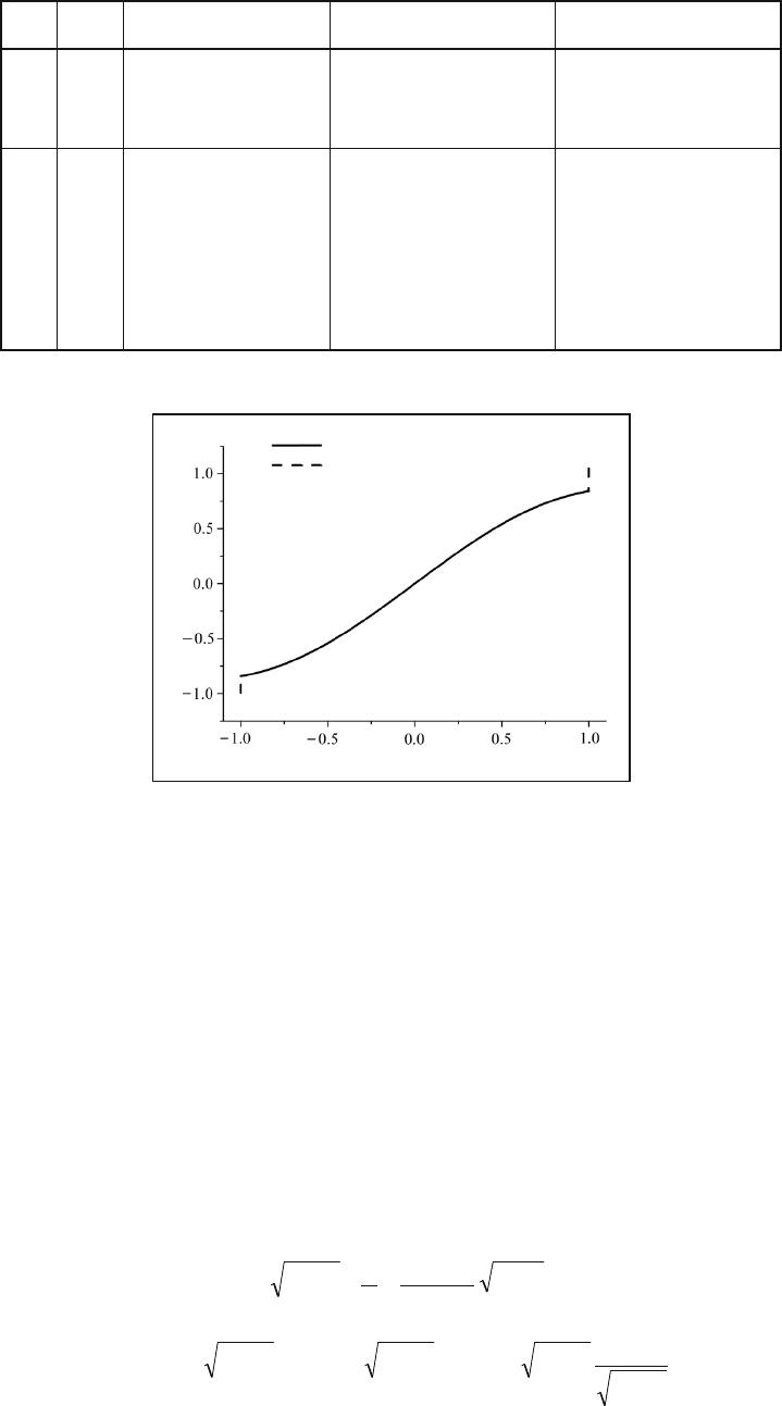
In Fig. 1, the plots of the functions

uy()

and

Re ( ( ))uy

n-2

are presented when

n =100

. As is easily seen, in the

middle of the interval

[,]-11

, the functions coincide with graphical accuracy; the number of exact significant figures in

the approximate solution in this region varies from three to seven. However, with approaching the end of the interval,

the real part of the error increases and its modulus remains equal to 0.208. The mean-square deviation of the modulus of

the difference between approximate and exact solutions equals 0.03 when

n =100

Thus, the results of application of the numerical method to the solution of model hypersingular integral

equation (21) of the second kind allow one to estimate and characterize the convergence of this method. In particular,

the convergence of the method is moderate and worsens with approaching the ends of the interval. Note that, in solving

applied problems of mathematical physics, for example, diffraction and wave scattering problems that lead to such

hypersingular integral equations, linear functionals of the solution of an integral equation should be constructed and

computed. This averages approximate solutions to a certain extent and provides average convergence that is rigorously

substantiated by inequality (20).

Problem 2. Consider now the following model hypersingular integral equation of the second kind on the

interval

[,]-11

hu y y

tdt()

()

=---+-

hy y y y y y

ch ch s hsin cos sin111

222

. (23)

403

TABLE 1

nj ut

()

-2

() |() ()|ut u t

1 0.837359 1.045342

3.56

0.208

2 0.794899 0.809269

1.31

0.015

3 0.659800 0.665980

7.69

6.23

4 0.386976 0.388816

3.41

1.87

1 0.840203 1.048468

1.36

0.208

2 0.828962 0.845430

4.48

0.016

3 0.800871 0.808066

7.69

7.21

4 0.746084 0.749143

3.21

3.08

5 0.653504 0.655318

2.33

1.83

6 0.515333 0.516286

1.56

9.66

7 0.331954 0.332487

9.10

5.41

8 0.114833 0.114974

2.94

1.44

Fig. 1

uy()

Re ( ( ))uy

n- 2

Solutions to Eq. (21)