
Generative Image Modeling Using Style
and Structure Adversarial Networks
Xiaolong Wang
(
B
)
and Abhinav Gupta
Robotics Institute, Carnegie Mellon University, Pittsburgh, USA
Abstract. Current generative frameworks use end-to-end learning and
generate images by sampling from uniform noise distribution. However,
these approaches ignore the most basic principle of image formation:
images are product of: (a) Structure: the underlying 3D model; (b) Style:
the texture mapped onto structure. In this paper, we factorize the image
generation process and propose Style and Structure Generative Adversar-
ial Network (S
2
-GAN). Our S
2
-GAN has two components: the Structure-
GAN generates a surface normal map; the Style-GAN takes the surface
normal map as input and generates the 2D image. Apart from a real vs.
generated loss function, we use an additional loss with computed surface
normals from generated images. The two GANs are first trained inde-
pendently, and then merged together via joint learning. We show our
S
2
-GAN model is interpretable, generates more realistic images and can
be used to learn unsupervised RGBD representations.
1 Introduction
Unsupervised learning of visual representations is one of the most fundamental
problems in computer vision. There are two common approaches for unsuper-
vised learning: (a) using a discriminative framework with auxiliary tasks where
supervision comes for free, such as context prediction [1,2] or temporal embed-
ding [3–8]; (b) using a generative framework where the underlying model is
compositional and attempts to generate realistic images [9–12]. The underlying
hypothesis of the generative framework is that if the model is good enough to
generate novel and realistic images, it should be a good representation for vision
tasks as well. Most of these generative frameworks use end-to-end learning to
generate RGB images from control parameters (z also called noise since it is sam-
pled from a uniform distribution). Recently, some impressive results [13]have
been shown on restrictive domains such as faces and bedrooms.
However, these approaches ignore one of the most basic underlying prin-
ciples of image formation. Images are a product of two separate phenomena:
Structure: this encodes the underlying geometry of the scene. It refers to the
underlying mesh, voxel representation etc. Style: this encodes the texture on the
objects and the illumination. In this paper, we build upon this IM101 principle of
image formation and factor the generative adversarial network (GAN) into two
generative processes as Fig. 1. The first, a structure generative model (namely
c
Springer International Publishing AG 2016
B. Leibe et al. (Eds.): ECCV 2016, Part IV, LNCS 9908, pp. 318–335, 2016.
DOI: 10.1007/978-3-319-46493-0
20

Generative Image Modeling using Style and Structure Adversarial Networks 319
Structure
GAN
Style
GAN
Uniform Noise
Distribution
Output1: Surface Normal
Uniform Noise
Distribution
Output2: Natural Indoor Scenes
(a) Generative Pipeline
(b) Generated Examples
(c) S
y
nthetic Scenes Renderin
g
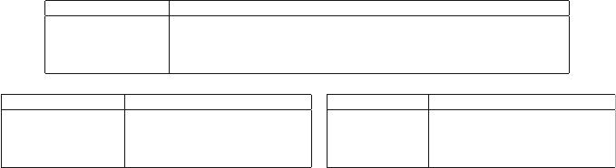
Fig. 1. (a) Generative Pipeline: Given ˆz sampled from uniform distribution, our
Structure-GAN generates a surface normal map as output. This surface normal map is
then given as input with ˜z to a second generator network (Style-GAN) and outputs an
image. (b) We show examples of generated surface normal maps and images. (c) Our
Style-GAN can be used as a rendering engine: given a synthetic scene, we can use it to
render a realistic image. To visualize the normals, we represent facing right with blue,
horizontal surface with green, facing left with red (blue → X; green → Y; red → Z).
(Color figure online)
Structure-GAN), takes ˆz and generates the underlying 3D structure (y
3D
) for the
scene. The second, a conditional generative network (namely Style-GAN), takes
y
3D
as input and noise ˜z to generate the image y
I
. We call this factored gener-
ative network Style and Structure Generative Adversarial Network (S
2
-GAN).
Why S
2
-GAN? We believe there are fourfold advantages of factoring the style
and structure in the image generation process. Firstly, factoring style and struc-
ture simplifies the overall generative process and leads to more realistic high-
resolution images. It also leads to a highly stable and robust learning procedure.
Secondly, due to the factoring process, S
2
-GAN is more interpretable as com-
pared to its counterparts. One can even factor the errors and understand where
the surface normal generation failed as compared to texture generation. Thirdly,
as our results indicate, S
2
-GAN allows us to learn RGBD representation in an
unsupervised manner. This can be crucial for many robotics and graphics appli-
cations. Finally, our Style-GAN can also be thought of as a learned rendering
engine which, given any 3D input, allows us to render a corresponding image.
It also allows us to build applications where one can modify the underlying 3D
structure of an input image and render a completely new image.
320 X. Wang and A. Gupta
However, learning S
2
-GAN is still not an easy task. To tackle this challenge,
we first learn the Style-GAN and Structure-GAN in an independent manner. We
use the NYUv2 RGBD dataset [14] with more than 200 K frames for learning the
initial networks. We train a Structure-GAN using the ground truth surface nor-
mals from Kinect. Because the perspective distortion of texture is more directly
related to normals than to depth, we use surface normal to represent image
structure in this paper. We learn in parallel our Style-GAN which is conditional
on the ground truth surface normals. While training the Style-GAN, we have two
loss functions: the first loss function takes in an image and the surface normals
and tries to predict if they correspond to a real scene or not. However, this loss
function alone does not enforce explicit pixel based constraints for aligning gen-
erated images with input surface normals. To enforce the pixel-wise constraints,
we make the following assumption: if the generated image is realistic enough, we
should be able to reconstruct or predict the 3D structure based on it. We achieve
this by adding another discriminator network. More specifically, the generated
image is not only forwarded to the discriminator network in GAN but also a
input for the trained surface normal predictor network. Once we have trained
an initial Style-GAN and Structure-GAN, we combine them together and per-
form end-to-end learning jointly where images are generated from ˆz, ˜z and fed
to discriminators for real/fake task.
2 Related Work
Unsupervised learning of visual representation is one of the most challenging
problems in computer vision. There are two primary approaches to unsupervised
learning. The first is the discriminative approach where we use auxiliary tasks
such that ground truth can be generated without labeling. Some examples of
these auxiliary tasks include predicting: the relative location of two patches [2],
ego-motion in videos [15,16], physical signals [17–19].
A more common approach to unsupervised learning is to use a generative
framework. Two types of generative frameworks have been used in the past.
Non-parametric approaches perform matching of an image or patch with the
database for tasks such as texture synthesis [20] or super-resolution [21]. In
this paper, we are interested in developing a parametric model of images. One
common approach is to learn a low-dimensional representation which can be used
to reconstruct an image. Some examples include the deep auto-encoder [22,23]or
Restricted Boltzmann machines (RBMs) [24–28]. However, in most of the above
scenarios it is hard to generate new images since sampling in latent space is not
an easy task. The recently proposed Variational auto-encoders (VAE) [10,11]
tackles this problem by generating images with variational sampling approach.
However, these approaches are restricted to simple datasets such as MNIST. To
generate interpretable images with richer information, the VAE is extended to
be conditioned on captions [29] and graphics code [30]. Besides RBMs and auto-
encoders, there are also many novel generative models in recent literature [31–34].
For example, Dosovitskiy et al. [31] proposed to use CNNs to generate chairs.
Generative Image Modeling using Style and Structure Adversarial Networks 321
In this work, we build our model based on the Generative Adversarial Net-
works (GANs) framework proposed by Goodfellow et al. [9]. This framework was
extended by Denton et al. [35] to generate images. Specifically, they proposed to
use a Laplacian pyramid of adversarial networks to generate images in a coarse
to fine scheme. However, training these networks is still tricky and unstable.
Therefore, an extension DCGAN [13] proposed good practices for training adver-
sarial networks and demonstrated promising results in generating images. There
are more extensions include using conditional variables [36–38]. For instance,
Mathieu et al. [37] introduced to predict future video frames conditioned on the
previous frames. In this paper, we further simplify the image generation process
by factoring out the generation of 3D structure and style.
In order to train our S
2
-GAN we combine adversarial loss with 3D surface
normal prediction loss [39–42] to provide extra constraints during learning. This
is also related to the idea of combining multiple losses for better generative
modeling [43–45]. For example, Makhzani et al. [43] proposed an adversarial
auto-encoder which takes the adversarial loss as an extra constraint for the latent
code during training the auto-encoder. Finally, the idea of factorizing image into
two separate phenomena has been well studied in [46–49], which motivates us
to decompose the generative process to structure and style. We use the RGBD
data from NYUv2 to factorize and learn a S
2
-GAN model.
3 Background for Generative Adversarial Networks
The Generative Adversarial Networks (GAN) [9] contains two models: generator
G and discriminator D. The generator G takes the input which is a latent random
vector z sampled from uniform noise distribution and tries to generate a realistic
image. The discriminator D performs binary classification to distinguish whether
an image is generated from G or it is a real image. Thus the two models are
competing against each other (hence, adversarial): network G will try to generate
images which will be hard for D to differentiate from real image, meanwhile
network D will learn to avoid getting fooled by G.
Formally, we optimize the networks using gradient descent with batch size M.
We are given samples as X =(X
1
, ..., X
M
) and a set of z sampled from uniform
distribution as Z =(z
1
, ..., z
M
). The training of GAN is an iterative procedure
with 2 steps: (i) fix the parameters of network G and optimize network D;
(ii) fix network D and optimize network G. The loss for training network D is,
L
D
(X, Z)=
M/2
i=1
L(D(X
i
), 1) +
M
i=M/2+1
L(D(G(z
i
)), 0). (1)
Inside a batch, half of images are real and the rest G(z
i
) are images generated by
G given z
i
. D(X
i
) ∈ [0, 1] represents the binary classification score given input
image X
i
. L(y
∗
,y)=−[y log(y
∗
)+(1− y)log(1 − y
∗
)] is the binary entropy loss.
Thus the loss Eq. 1 for network D is optimized to classify the real image as label
322 X. Wang and A. Gupta
Table 1. Network architectures. Top: generator of Structure-GAN; bottom: discrimi-
nator of Structure-GAN (left) and discriminator of Style-GAN (right). “conv” means
convolutional layer, “uconv” means fractionally-strided convolutional (deconvolutional)
layer, where 2(up) stride indicates 2x resolution. “fc” means fully connected layer.
Structure-GAN(G) fc uconv conv conv conv conv uconv conv uconv conv
Input Size − 9 18181818 18 36 36 72
Kernel Number 9 × 9 × 64 128 128 256 512 512 256 128 64 3
Kernel Size − 433334345
Stride − 2(up)1 1 1 12(up)12(up)1
Structure-GAN(D) conv conv conv conv conv fc
Input Size 72 36 36 18 9 −
Kernel Number 64 128 256 512 128 1
Kernel Size 55333−
Stride 21221−
Style-GAN(D) conv conv conv conv conv fc
Input Size 128 64 32 16 8 −
Kernel Number 64 128 256 512 128 1
Kernel Size 55333−
Stride 22221−
1 and the generated image as 0. On the other hand, the generator G is trying to
fool D to classify the generated image as a real image via minimizing the loss:
L
G
(Z)=
M
i=M/2+1
L(D(G(z
i
)), 1). (2)
4 Style and Structure GAN
GAN and DCGAN approaches directly generate images from the sampled z.
Instead, we use the fact that image generation has two components: (a) gener-
ating the underlying structure based on the objects in the scene; (b) generating
the texture/style on top of this 3D structure. We use this simple observation
to decompose the generative process into two procedures: (i) Structure-GAN -
this process generates surface normals from sampled ˆz and (ii) Style-GAN - this
model generates the images taking as input the surface normals and another
latent variable ˜z sampled from uniform distribution. We train both models with
RGBD data, and the ground truth surface normals are obtained from the depth.
4.1 Structure-GAN
We can directly apply GAN framework to learn how to generate surface normal
maps. The input to the network G will be ˆz sampled from uniform distribution
and the output is a surface normal map. We use a 100-d vector to represent the
ˆz and the output is in size of 72 × 72 × 3 (Fig. 2). The discriminator D will learn
to classify the generated surface normal maps from the real maps obtained from
depth. We introduce our network architecture as following.
Generator Network. As Table 1 (top row) illustrates, we apply a 10-layer
model for the generator. Given a 100-d ˆz as input, it is first fully connected to a
3D block (9×9×64). Then we further perform convolutional operations on top of
Generative Image Modeling using Style and Structure Adversarial Networks 323
Fig. 2. Left: 4 Generated Surface Normal maps. Right: 2 Pairs of rendering results on
ground truth surface normal maps using the Style-GAN without pixel-wise constraints.
it and generate the surface normal map in the end. Note that “uconv” represents
fractionally-strided convolution [13], which is also called as deconvolution. We
follow the settings in [13] and use Batch Normalization [50] and ReLU activations
after each layer except for the last layer, where a TanH activation is applied.
Discriminator Network. We show the 6-layer network architecture in Table 1
(bottom left). Taking an image as input, the network outputs a single num-
ber which predicts the input surface normal is real or generated. We use
LeakyReLU [51,52] for activation functions as in [13]. However, we do not apply
Batch Normalization here. In our case, we find that the discriminator network
easily finds trivial solutions with Batch Normalization.
4.2 Style-GAN
Given the RGB images and surface normal maps from Kinect, we train another
GAN in parallel to generate images conditioned on surface normals. We call this
network Style-GAN. First, we modify our generator network to a conditional
GAN as proposed in [35,36]. The conditional information, i.e., surface normal
maps, are given as additional inputs for both the generator G and the discrim-
inator D. Augmenting surface normals as an additional input to D not only
forces the generated image to look real, but also implicitly enforces the gener-
ated image to match the surface normal map. While training this discriminator,
we only consider real RGB images and their corresponding surface normals as
the positive examples. Given more cues from surface normals, we generate higher
resolution of 128 × 128 × 3 images with the Style-GAN.
Formally, we have a batch of RGB images X =(X
1
, ..., X
M
) and their corre-
sponding surface normal maps C =(C
1
, ..., C
M
), as well as samples from noise
distribution
˜
Z =(˜z
1
, ..., ˜z
M
). We reformulate the generative function from G(˜z
i
)
to G(C
i
, ˜z
i
) and discriminative function is changed from D(X
i
)toD(C
i
,X
i
).
Then the loss of discriminator network in Eq. 1 can be reformulated as,
L
D
cond
(X, C ,
˜
Z)=
M/2
i=1
L(D(C
i
,X
i
), 1) +
M
i=M/2+1
L(D(C
i
,G(C
i
, ˜z
i
)), 0), (3)
and the loss of generator network in Eq. 2 can be reformulated as,
L
G
cond
(C,
˜
Z)=
M
i=M/2+1
L(D(C
i
,G(C
i
, ˜z
i
)), 1). (4)
324 X. Wang and A. Gupta
64
64
64
32
32
128
128
128
64
8
8
64
16
16
32
32
256
5x5
conv
64
5x5
conv
4x4
uconv
4x4
uconv
3x3
conv
3x3
conv
3x3
conv
4x4
uconv
4x4
uconv
4x4
uconv
5x5
conv
32
32
16
16
512
512
16
16
256
32
32
128
64
64
64
128
128
128
128
Concat
100
fc
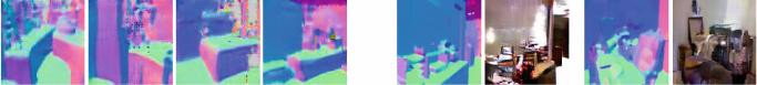
Fig. 3. The architecture of the generator in Style-GAN.
Style
Generator
Network
Fully
Convolutional
Network
Style
Discriminator
Network
Binary
Classification
Input
Surface Normal
Estimation
Generated
Images
Real
Images
Uniform Noise
Distribution
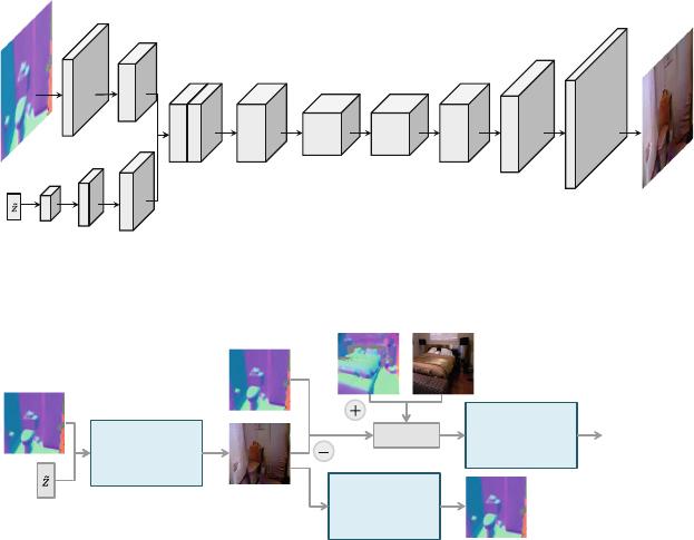
Fig. 4. Our Style-GAN. Given the ground truth surface normals and ˜z as inputs,
the generator G learns to generate RGB images. The supervision comes from two
networks: The discriminator network takes the generated images, real images and their
corresponding normal maps as inputs to perform classification; The FCN takes the
generated images as inputs and predict the surface normal maps.
We apply the same scheme of iterative training. By doing this, we can gen-
erate the images with network G as visualized in Fig. 2 (right).
Network Architecture. We show our generator as Fig. 3. Given a 128×128×3
surface normal map and a 100-d ˜z as input, they are firstly forwarded to convo-
lutional and deconvolutional layers respectively and then concatenated to form
32 × 32 × 192 feature maps. On top of these feature maps, 7 layers of convolu-
tions and deconvolutions are further performed. The output of the network is a
128 × 128 × 3 RGB image. For the discriminator, we apply the similar architec-
ture of the one in Structure-GAN (bottom right in Table 1). The input for the
network is the concatenation of surface normals and images (128 × 128 × 6).
4.3 Multi-task Learning with Pixel-Wise Constraints
The Style-GAN can make the generated image look real and also enforce it to
match the provided surface normal maps implicitly. However, as shown Fig. 2,the
images are noisy and the edges are not well aligned with the edges in the surface
normal maps. Thus, we propose to add a pixel-wise constraint to explicitly guide
the generator to align the outputs with the input surface normal maps.
Generative Image Modeling using Style and Structure Adversarial Networks 325
Style
Generator
Network
Style
Discriminator
Network
Generated
Images
Structure
Generator
Network
Structure
Discriminator
Network
Uniform Noise
Distribution
Uniform Noise
Distribution
Generated
Normals
Generated
Normals
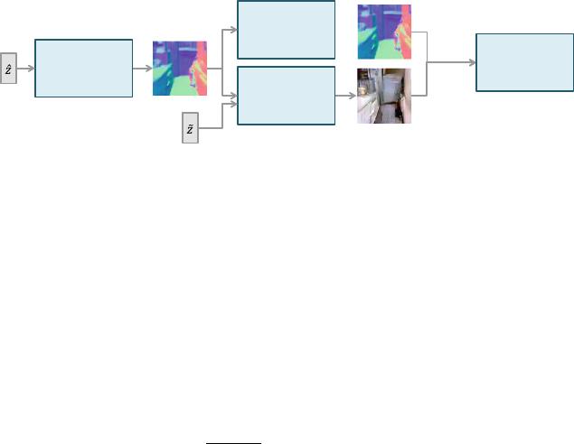
Fig. 5. Full model of our S
2
-GAN. It can directly generate RGB images given ˆz, ˜z as
inputs. For simplicity, we do not visualize the positive samples in training. During joint
learning, the loss from Style-GAN is also passed down to the Structure-GAN.
We make the following assumption: If the generated image is real enough,
it can be used for reconstructing the surface normal maps. To encode this con-
straint, we train another network for surface normal estimation. We modify the
Fully Convolutional Network (FCN) [53] with the classification loss as men-
tioned in [39] for this task. More specifically, we quantize the surface normals to
40 classes with k-means clustering as in [39,54] and the loss is defined as
L
FCN
(X, C)=
1
K × K
M
i=1
K×K
k=1
L
s
(F
k
(X
i
),C
i,k
), (5)
where L
s
means the softmax loss and the output surface normal map is in K ×K
dimension, and K = 128 is in the same size of input image. F
k
(X
i
) is the output
of kth pixel in the ith sample. C
i,k
(1 C
i,k
40) is the label for the kth pixel in
sample i. Thus the loss is designed to enforce each pixel in the image to generate
accurate surface normal. Note that when training the FCN, we use the RGBD
data which provides indoor scene images and ground truth surface normals. The
model is trained from scratch without ImageNet pre-training.
FCN Architecture. We apply the AlexNet [55] following the same training
scheme as [53], with modifications on the last 3 layers. Given a generated 128 ×
128 image, it is first upsampled to 512×512 before feeding into the FCN. For the
two layers before the last layer, we use smaller kernel numbers of 1024 and 512.
The last layer is a deconvolutional layer with stride 2. In the end, upsampling
(4x resolution) is further applied to generate the high quality results.
Given the trained FCN model, we can use it as an additional supervision
(constraint) in the adversarial learning. Our final model is illustrated in Fig. 4.
During training, not only the gradients from the classification loss of D will be
passed down to G, but also the surface normal estimation loss from the FCN is
passed through the generated image to G. This way, the adversarial loss from
D will make the generated images look real, and the FCN will give pixel-wise
constraints to make the generated images aligned with surface normal maps.
Formally, we combine the two losses in Eqs. 4 and 5 for the generator G,
L
G
multi
(C,
˜
Z)=L
G
cond
(C,
˜
Z)+L
FCN
(G(C,
˜
Z), C ), (6)
326 X. Wang and A. Gupta
where G(C,
˜
Z) represents the generated images given a batch of surface normal
maps C and noise
˜
Z. The training procedure for this model is similar to the
original adversarial learning, which includes three steps in each iteration:
– Fix the generator G, optimize the discriminator D with Eq. 3.
– Fix the FCN and the discriminator D, optimize the generator G with Eq. 6.
– Fix the generator G, fine-tune FCN using generated and real images.
Note that the parameters of FCN model are fixed in the beginning of multi-
task learning, i.e., we do not fine-tune FCN in the beginning. The reason is the
generated images are not good in the beginning, so feeding bad examples to FCN
seems to make the surface normal prediction worse.
4.4 Joint Learning for S
2
-GAN
After training the Structure-GAN and Style-GAN independently, we merge all
networks and train them jointly. As Fig. 5 shows, our full model includes surface
normal generation from Structure-GAN, and based on it the Style-GAN gener-
ates the image. Note that the generated normal maps are first passed through
an upsampling layer with bilinear interpolation before they are forwarded to the
Style-GAN. Since we do not use ground truth surface normal maps to generate
the images, we remove the FCN constraint from the Style-GAN. The discrim-
inator in Style-GAN takes generated normals and images as negative samples,
and ground truth normals and real images as positive samples.
For the Structure-GAN, the generator network receives not only the gradients
from the discriminator of Structure-GAN, but also the gradients passed through
the generator of Style-GAN. In this way, the network is forced to generate surface
normals which not only are realistic but also help generate better RGB images.
Formally, the loss for the generator network of Structure-GAN can be represented
as combining Eqs. 2 and 4,
L
G
joint
(
ˆ
Z,
˜
Z)=L
G
(
ˆ
Z)+λ · L
G
cond
(G(
ˆ
Z),
˜
Z) (7)
where
ˆ
Z =(ˆz
1
, ..., ˆz
M
)and
˜
Z =(˜z
1
, ..., ˜z
M
) represent two sets of samples drawn
from uniform distribution for Structure-GAN and Style-GAN respectively. The
first term in Eq. 7 represents the adversarial loss from the discriminator of
Structure-GAN and the second term represents that the loss of the Style-GAN
is also passed down. We set the coefficient λ =0.1 and smaller learning rate for
Structure-GAN than Style-GAN in the experiments, so that we can prevent the
generated normals from over fitting to the task of generating RGB images via
Style-GAN. In our experiments, we find that without constraining λ and learn-
ing rates, the loss L
G
(
ˆ
Z) easily diverges to high values and the Structure-GAN
can no longer generate reasonable surface normal maps.
5 Experiments
We perform two types of experiments: (a) We qualitatively and quantitatively
evaluate the quality of images generates using our model; (b) We evaluate the
Generative Image Modeling using Style and Structure Adversarial Networks 327
quality of unsupervised representation learning by applying the network for dif-
ferent tasks such as image classification and object detection.
Dataset. We use the NYUv2 dataset [14] in our experiment. We use the raw
video data during training and extract 200 K frames from the 249 training video
scenes. We compute the surface normals from the depth as [39,42].
Parameter Settings. We follow the parameters in [13] for training. We trained
the models using Adam optimizer [56] with momentum term β
1
=0.5,β
2
=0.999
and batch size M = 128. The inputs and outputs for all networks are scaled to
[−1, 1] (including surface normals and RGB images). During training the Style
and Structure GANs separately, we set the learning rate to 0.0002. We train the
Structure-GAN for 25 epochs. For Style-GAN, we first fix the FCN model and
train it for 25 epochs, then the FCN model are fine-tuned together with 5 more
epochs. For joint learning, we set learning rate as 10
−6
for Style-GAN and 10
−7
for Structure-GAN and train them for 5 epochs.
Baselines. We have 4 baseline models trained on NYUv2 training set:
(a) DCGAN [13]: it takes uniform noise as input and generate 64 × 64 images;
(b) DCGAN + LAPGAN: we train a LAPGAN [35] on top of DCGAN, which
takes lower resolution images as inputs and generates 128 × 128 images. We
apply the same architecture as our Style-GAN for LAPGAN (Fig. 3 and Table 1).
(c) DCGANv2: we train a DCGAN with the same architecture as our Structure-
GAN (Table 1). (d) DCGANv2+LAPGAN: we train another LAPGAN on top
of DCGANv2 as (b) with the same architecture. Note that baseline (d) has the
same model complexity as our model.
5.1 Qualitative Results for Image Generation
Style-GAN Visualization. Before showing the image generation results of
the full S
2
-GAN model, we first visualize the results of our Style-GAN given the
ground truth surface normals on the NYUv2 test set. As illustrated in the first
3 rows of Fig. 6, we can generate nice rendering results which are well aligned
with the surface normal inputs. By comparing with the original RGB images, we
show that our method can generate a different style (illumination, color, texture)
of image with the same structure. We also make comparisons on the results of
Style-GAN with/without pixel-wise constraints as visualized in Fig. 7. We show
that if we train the model without the pixel-wise constraint, the output is less
smooth and noisier than our approach.
Rendering on Synthetic Scenes. One application of our Style-GAN is ren-
dering synthetic scenes. We use the 3D models annotated in [57] to generate the
synthetic scenes. We use the scenes corresponding to the NYUv2 test set and
make some modifications by rotation, zooming in/out. As the last two rows of
Fig. 6 show, we can obtain very realistic rendering results on 3D models.
S
2
-GAN Visualization. We now show the results of our full generative model.
Given the noise ˆz, ˜z, our model generate both surface normal maps (72×72) and
