
Vol.:(0123456789)
Environmental and Resource Economics
https://doi.org/10.1007/s10640-020-00472-7
1 3
Optimal Siting, Sizing, andEnforcement ofMarine Protected
Areas
H.J.Albers
1
· L.Preonas
2
· T.Capitán
3
· E.J.Z.Robinson
4
· R.Madrigal‑Ballestero
5
Accepted: 9 July 2020
© The Author(s) 2020
Abstract
The design of protected areas, whether marine or terrestrial, rarely considers how people
respond to the imposition of no-take sites with complete or incomplete enforcement. Con-
sequently, these protected areas may fail to achieve their intended goal. We present and
solve a spatial bio-economic model in which a manager chooses the optimal location, size,
and enforcement level of a marine protected area (MPA). This manager acts as a Stackel-
berg leader, and her choices consider villagers’ best response to the MPA in a spatial Nash
equilibrium of fishing site and effort decisions. Relevant to lower income country settings
but general to other settings, we incorporate limited enforcement budgets, distance costs of
traveling to fishing sites, and labor allocation to onshore wage opportunities. The optimal
MPA varies markedly across alternative manager goals and budget sizes, but always induce
changes in villagers’ decisions as a function of distance, dispersal, and wage. We consider
MPA managers with ecological conservation goals and with economic goals, and iden-
tify the shortcomings of several common manager decision rules, including those focused
on: (1) fishery outcomes rather than broader economic goals, (2) fish stocks at MPA sites
rather than across the full marinescape, (3) absolute levels rather than additional values,
and (4) costless enforcement. Our results demonstrate that such naïve or overly narrow
decision rules can lead to inefficient MPA designs that miss economic and conservation
opportunities.
Keywords Additionality· Bio-economic model· Enforcement· Leakage· Nash
equilibrium· No-take reserves· Park effectiveness· Reserve site selection· Spatial
prioritization· Systematic conservation planning· Marine spatial planning
1 Introduction
Many countries are expanding their protected area (PA) networks, terrestrial and marine, to
achieve both ecological goals, which often align with international conservation agreements
(Pereira etal. 2013), and economic goals (Gaines etal. 2010; Jentoft etal. 2011), which often
prioritize sustainable resource management for the benefit of nearby resource-dependent
* H. J. Albers
Extended author information available on the last page of the article

H.J.Albers et al.
1 3
communities (Cabral etal. 2019; Carr et al. 2019). However, for any of these goals, eco-
nomic efficiency requires that PA siting and management decisions anticipate and consider
the response of potential resource extractors, especially in settings of limited enforcement
budgets (Cabral etal. 2017). Empirical economic analyses of terrestrial park effectiveness
often rely on von Thunen-inspired models to predict the level of deforestation that would
occur if a location was not in a PA, and then calculate the level of “avoided deforestation”
created by the PA as a measure of its effectiveness (e.g. Pfaff et al. 2014). Working from
the opposite starting point, we use a model of villagers’ fishing site and labor decisions to
predict how villagers react to a marine protected area (MPA), and incorporate these vil-
lager best responses into optimal MPA design to determine the optimal size, location, and
enforcement of an MPA intended to maximize either ecological or economic objectives.
To predict how villagers react to an MPA, we develop a game-theoretic model in which
villagers make individual fishing site and labor effort decisions that aggregate through a
Nash equilibrium with spatially explicit micro-foundations. To be general to lower-income
country settings, we explicitly model labor allocation decisions across fishing and non-
fishing income-generating activities and a fishing site choice, rather than allocating fishing
effort until achieving rent dissipation in each fishing site (Sanchirico and Wilen 2001).
1
By modeling fixed distance costs of traveling to each potential fishing site, we incorporate
the spatial interactions between fishers’ site choice and managers’ MPA size, sites, and
enforcement decisions (Robinson etal. 2014; Madrigal-Ballestero etal. 2017). Specifically,
we model biologically homogeneous fishing sites with density dispersal across sites, but
heterogeneous distance costs induce heterogeneous returns to fishing across sites. Finally,
acting as a Stackelberg leader and to maximize a specific goal, our manager chooses the
optimal size, sites, and enforcement level considering villagers’ spatial equilibrium best
responses to the MPA.
MPAs are often used for fisheries management and ecological conservation goals,
including ecological objectives around fish populations or marine biodiversity and eco-
nomic goals around livelihood objectives and fish yields (Batista etal. 2011; Pajaro etal.
2010; Pomeroy etal. 2005). To reflect the varied objectives for MPAs worldwide, we con-
sider two central goals: maximize income as an economic goal and maximize the avoided
fish stock losses in the marinescape as an ecological goal. Our economic goal emphasizes a
broad objective similar to maximizing welfare, rather than following the fishery economics
literature’s emphasis on aggregate yield and fishery profits, because aggregate income is
inclusive of fishery profits and onshore wage earnings.
2
Our ecological goal of maximiz-
ing avoided stock losses in the marinescape corresponds with the systematic conservation
planning literature’s emphasis on evaluating conservation policy at the landscape level and
on the additional conservation created.
3
Regardless of the manager’s goal, we consider the optimal MPA design both when a
manager is constrained by an enforcement budget and when this constraint does not bind.
By considering the budget-constrained managers, we can address a central issue for PAs
1
This approach allows us to address income considerations both in fishing and outside of fishing, labor
allocation decisions that determine fishery exit, and settings without rent dissipation, as in related work
(Albers etal. 2020). In the cases presented in this paper, all the results lead to rent dissipation after covering
the fixed costs of distance. We maintain Sanchirico and Wilen’s assumption that non-MPA sites (patches)
are open-access.
2
We also consider the optimal MPAs for a yield or fishery profit maximizing goal.
3
Here, “avoided fish stock loss” is akin to the “avoided deforestation” in the terrestrial park evaluation
literature (i.e. additionality).

Optimal Siting, Sizing, andEnforcement ofMarine Protected…
1 3
in lower-income countries: PAs without sufficient enforcement become “paper parks”
that provide few additional PA benefits because people continue to extract resources
(e.g. Adams etal. 2019; Brown et al. 2018; Bonham et al. 2008). In our model, villag-
ers’ respond to the “carrot” of MPA configuration’s impact on dispersal (i.e. increased fish
stocks in a particular site) and to the “stick” of the MPA’s potentially incomplete enforce-
ment (i.e. increased probability of being caught and losing their harvest), in addition to
other characteristics of the setting. We find that the optimal MPA differs markedly across
management goals and non-monotonically across budgets in ways that reflect the villagers’
spatially explicit response, in the form of a spatial Nash equilibrium, to the MPA at the
long run steady state fish stock. Previous studies that consider enforcement costs and the
response to incomplete enforcement in making MPA siting decisions either conduct that
analysis with assumptions about constant fishing effort (Byers and Noonburg 2007) or in
an implicitly spatial setting without modeling distance as a component of the fishers’ site
choice (Yamazaki etal. 2014).
Furthermore, we show the potential shortcomings of establishing an MPA based on
often-used goals that do not consider either the full livelihood of the villagers (i.e. fish-
ing income and non-fishing income) or the full marinescape (i.e. stock inside and outside
the MPA). First, while the economics literature on marine protection typically considers
only economic outcomes within fisheries (e.g. Smith and Wilen 2003), MPAs may shift
labor out of fishing and into other sectors of the economy. By introducing onshore wage
labor as an outside option, we can compare the standard goal of yield-maximization with a
more holistic goal of maximizing income for the villagers (i.e. a better measure of welfare).
By allowing for onshore wage labor and constraining the manager’s enforcement capac-
ity, our model highlights the distinction between yield- and income-maximization that is
particularly salient in low- and middle-income countries where artisanal fishers frequently
work multiple jobs and limited enforcement capacity cannot completely deter illegal har-
vest. Second, while ecological conservation goals typically focus on outcomes within the
geographic footprint of the PA itself, incomplete enforcement can cause economic activ-
ity to spillover to nearby areas just outside the enforced zone (Robalino etal. 2017) and
fish dispersal from sites of high relative fish density influence fishing site decisions such
as “fishing the line” (Kellner etal. 2007). If a naïve manager designs an MPA to maxi-
mize avoided stock loss only within the MPA itself, spillovers to adjacent fishing sites are
likely to undermine its ecological impact across the full marinescape. By explicitly mod-
eling how both fish and people move across space, including across MPA borders, we com-
pare standard ecological MPA-focused goals with a broader objective to maximize avoided
stock loss across the full marinescape.
Our results reveal qualitative and quantitative differences in optimal MPAs established
to achieve different goals; show changes in MPA design across budget levels; elucidate
relationships between enforcement levels and MPA outcomes; and inform a policy discus-
sion. Specifically, we make three main contributions. First, we extend the economic analy-
sis of MPAs by including multiple sites and spatially explicit modeling of villager labor
and site decisions with heterogeneous distance costs and incomplete enforcement. Second,
we extend the systematic conservation planning and reserve site selection literatures by
including a model of fishers’ MPA response directly in the decision framework for select-
ing MPA sites. Third, by incorporating constrained enforcement budgets, our results speak
to real-world challenges faced by PA managers. This article continues with the develop-
ment of a model that considers several manager goals. Section III presents the open access
decisions of villagers in IIIA, the optimal MPAs from a manager who maximizes income
and one who maximizes avoided stock loss across the marinescape in IIIB, and interprets

H.J.Albers et al.
1 3
those results in IIIC. Section IV reports and interprets the MPA results of 3 “naïve” manag-
ers. Section V discusses the policy implications of the results and section VI concludes.
2 Model
2.1 Overview
We develop a spatial bio-economic model to study the MPA manager’s siting, sizing,
and enforcement level decisions, given the presence of villagers who either fish or work
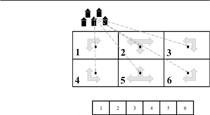
onshore. First, we define our stylized marinescape spatial setting as an
R × C
matrix with a
village located next to the first site (Fig.1). The biological part of the model is a fish meta-
population structure with density dispersal. The economic part of the model includes two
types of participants:
N
identical villagers and one manager. As the Stackelberg leader, the
manager defines the MPA, comprised of no-take sites within the marinescape and the level
of enforcement that maximizes the manager’s goal, considering both fish dynamics and
the villagers’ equilibrium response. Each individual villager allocates labor across onshore
wage labor and fishing labor to maximize their individual income. Each villager considers
the other villagers’ choices, the location and level of enforcement within the MPA, distance
costs, and fish stocks per site, which results in a spatial Nash equilibrium that constitutes
the villagers’ best response to the Stackelberg leader’s MPA.
2.2 Fish Dynamics
In common with much of the marine economics literature, we define the biological and
spatial setting as a fish metapopulation structure with adult fish density dispersal across the
R × C
marinescape. A fishing site,
i
, is one cell in that matrix, indexed from
1
to
(R
⋅
C)
.
Cells—or fishing sites—in the first row,
i ∈
{
1, … , C
}
, are closest to the shore (see Fig.1).
Fish net growth, harvest, and dispersal over time change the fish stock in each site:
where
X
t
is a
(
R
⋅
C
)
× 1
vector of fish stocks over fishing sites
x
i
at time
t
,
K
is a
(
R
⋅
C
)
× 1
vector of site carrying capacities,
D
is a
(
R
⋅
C
)
×
(
R
⋅
C
)
dispersal matrix, and
H
t
is a
(
R
⋅
C
)
× 1
vector of the sum of all individual fishers’ harvests from each site
i
at time
t
.
The logistic function
G
(X
t
, K)=gX
t
(
1 −
X
t
K
)
depicts natural population net growth at each
specific site, with
g
indicating the intrinsic net growth rate. The dispersal matrix
D
opera-
tionalizes the density dependent dispersal process as a linear function of fish stocks of all
sites with net dispersal to lower density neighbors that share a boundary through rook con-
tiguity (Sanchirico and Wilen 2001; Albers etal. 2015; see Appendix 1). Our results hold
in the steady state stock of fish,
X
SS
, which occurs when
X
t
= X
t+𝟏
.
2.3 Manager Decisions
Each manager selects sites to define an MPA that maximizes either an economic or an
ecological goal. First, for the economic goal, we posit a manager who maximizes total
income from fishing and non-fishing activities. This goal aligns with the objective func-
tion of a benevolent social planner and many lower income country managers (Carr etal.
(1)
X
t
+
𝟏
= X
t
+ G
(
X
t
, K
)
+ DX
t
− H
t
,

Optimal Siting, Sizing, andEnforcement ofMarine Protected…
1 3
2019; Madrigal-Ballestero etal. 2017). Consistent with the optimal enforcement literature,
the income-maximizing manager accounts for both legal and illegal harvest (Stigler 1970;
Milliman 1986).
4
Second, for the ecological goal, we posit a manager who maximizes
avoided aggregate fish stock losses (ASL) across the marinescape, recognizing the fun-
damental role that fish dispersal plays across the marinescape (Jentoft etal. 2011; Pressey
and Bottrill 2009). This ASL-marinescape manager considers both the spatial leakage of
fishing effort that generates stock losses in non-MPA sites and fish dispersal across MPA
borders. In addition, this manager’s goal considers the additional benefits created by the
MPA through the focus on “avoided stock loss” (Andam etal. 2008; Pfaff etal. 2014). The
managers choose the size of the MPA (i.e. number of sites in the MPA) and the specific
location of the MPA sites, creating an
(
R
⋅
C
)
× 1
element vector, S, where each element of
the vector depicts whether that site is within the MPA:
The manager chooses one level of enforcement that is constant throughout the MPA at
level
𝜙 ∈
[
0, 1
]
, where
𝜙 = 1
denotes complete enforcement and implies a probability of
being caught and punished of 1.
5
Following the optimal enforcement literature, managers
incur enforcement costs,
𝛽
, which here follow a linear and additive form with marginal cost
c
per unit
𝜙
per unit (Nostbakken 2008; Milliman 1986; Sutinen and Andersen 1985):
Each manager accounts for the villagers’ optimal responses to the MPA; thus, the man-
ager optimizes over the outcome of villagers’ Nash equilibrium location and labor choices
in response to the MPA at the steady state for fish stocks.
The income-maximizing manager’s decision is:
The ASL-marinescape maximizing manager’s decision is:
s
i
=
{
1 if site i is in the MPA
0 otherwise
.
𝛽
=
∑
i
s
i
[c𝜙
]
max
S,𝜙
∑
i
pH
i
(1 − 𝜙
i
)+
∑
n
w
(
l
w,n
)
𝛾
,
4
The optimal enforcement economics literature and practical input from managers state that managers
focus on the full social value of harvested fish—including both legal and illegal harvest in their values—
although managers use a penalty of lost time and extraction when villagers are caught harvesting illegally
(Stigler 1970; Milliman 1986).
5
We limit the manager to one level of enforcement throughout the MPA for computational and exposi-
tional ease. That constant level of enforcement reflects some settings that require all locations in a PA to
be treated equally (e.g. Albers 2010). Related research with this model (Albers etal. 2015) and with terres-
trial models (Albers 2010; Albers and Robinson 2011, 2013) demonstrates that lower levels of enforcement
probability are needed to deter illegal harvest in sites that are more distant, and Albers etal. (2019) defines
optimal enforcement levels for each reserve in a terrestrial reserve network. Appendix D presents one case
of enforcement distance costs that finds that reducing enforcement costs near the village leads to MPAs
closer to the village and that these lower near-village costs enable managers to achieve their MPA goals
at lower budgets. Albers etal. (2020) considers enforcement distance costs in a similar marinescape with
1-site MPAs. In addition, based on fieldwork, the impact of distance costs on villager site choices appears
large relative to the impact of distance costs on patrolling decisions, especially in the marine setting with
guards in motorboats and artisanal fishers in dhows.
H.J.Albers et al.
1 3
where
x
i,OA
depicts the open access equilibrium and steady state stock value in site
i
,
p
is
the exogenous price of fish per unit harvest,
l
w,n
is the villager
n
’s allocation of onshore
wage labor,
w
is the exogenous onshore wage, and
𝛾 ∈
(
0, 1
)
creates diminishing returns to
onshore labor (reflecting imperfect labor markets). Both managers make these maximiza-
tion decisions subject to fish dispersal (Eq.1) and the best response of the villagers’ opti-
mization and Nash equilibrium, which determine
H
and
X
. To consider a lower income
country setting, we evaluate the managers’ decisions subject to an enforcement budget con-
straint:
B ≥ 𝛽.
To reflect common goals of the fishery economics literature, systematic conserva-
tion literature, conservation economics literature, and lower income country regional
development and conservation managers, we also consider several “naïve” managers
who do not consider the entire setting in their decisions. First, a naïve manager with an
economic goal maximizes the yield or the fishery profits from the marinescape but dis-
regards the MPA’s impact on total income. Second, two other naïve managers with eco-
logical goals consider only the stock inside the MPA: An ASL-MPA manager considers
only the avoided stock loss within the MPA rather than considering the marinescape,
and an MPA-stock manager maximizes the fish stock within the MPA rather than con-
sidering the additional benefits created by the MPA.
The yield-maximizing manager’s decision is:
The ASL-MPA maximizing manager’s decision is:
The MPA-stock maximizing manager’s decision is:
max
S,𝜙
∑
i
[x
i
− x
i,OA
]
,
max
S,𝜙
∑
i
H
i
(1 − 𝜙
i
)
max
S,𝜙
∑
i
s
i
[x
i
− x
i,OA
]
Fig. 1 Spatial setting. The
dashed lines represent the
distance from the village to each
fishing site and the wide arrows
show the dispersal of the fish
within the marinescape. The vec-
tor below the marinescape figure
corresponds to the vectorization
of the marinescape matrix

Optimal Siting, Sizing, andEnforcement ofMarine Protected…
1 3
We also consider two naïve managers—one based on the ASL-marinescape maximizer
and one based on the income-maximizer—who make MPA decisions assuming either that
their budget is large enough to induce complete deterrence or that their MPA automatically
produces complete deterrence.
2.4 Villagers
We include one village with
N
identical villagers who have full information about the MPA
and the resource setting. Each villager,
n
, seeks to maximize income by allocating labor
across two activities: fishing and onshore wage labor. This labor allocation framework
reflects the reality that many villagers allocate time across several activities, including
between fishing and tourism-related activities (Muthiga 2009; Madrigal-Ballestero et al.
2017) and between fishing and subsistence agriculture (Rahman etal. 2012; Robinson etal.
2014).
6
To achieve his goal, each villager chooses either to not fish at all, or to fish in one
site; and if the latter, how much time to fish, how much time to work onshore, and the fish-
ing site. Each villager recognizes that he has a fixed amount of labor time (
L
n
) to allocate
to working onshore (
l
w
), fishing in a given site (
l
f ,i
), and traveling in his boat from the vil-
lage to the fishing site (
l
d
(
i
)
):
Labor time in fishing represents the marginal cost of fishing and labor time for travel
to a fishing site captures the fixed distance costs of fishing, both valued at the opportunity
cost of time (i.e. the onshore wage). Fishing sites in our model differ due to two types of
spatial heterogeneity, in contrast with the standard spatially homogeneous frameworks (e.g.
Sanchirico and Wilen 2001). First, each fishing site is located at a different distance from
the village, inducing heterogeneous travel costs
l
d(i)
. Second, fish dispersal patterns are spa-
tially explicit, inducing heterogeneous returns to fishing across sites.
We assume a standard harvest function:
where an individual villager’s harvest in a given site i,
h
i,n
,
depends on the amount of labor
time that villager allocates to fishing in the site (
l
f ,i,n
)
as the marginal cost of fishing, the
stock of fish in the site, (
x
i
), and the catchability coefficient (
q
). The individual villager’s
harvest does not directly depend on the number of other villagers in the site (i.e. no conges-
tion costs), but it indirectly depends on the other villagers’ harvest in the site through the
steady state equilibrium stock effect, as in Eq.1. The total harvest in a given site is the sum
of all villagers’ harvests in the site i:
max
S,𝜙
∑
i
s
i
[x
i
]
(2)
L
n
≥ l
w,n
+ l
f ,i,n
+ l
d
(
i
)
,n
.
(3)
h
i,n
= l
f ,i,n
x
i
q,
(4)
H
i
=
∑
n
h
i,
n
6
Settings in which fishers have no alternative livelihood opportunities (e.g. Nayak 2017) correspond to a
zero-wage scenario in this model.

H.J.Albers et al.
1 3
Dynamic stock effects occur through the impact of the total harvest on the state variable
x
i
(an element of
X
in the equation of fish dynamics) in the steady state. Given this inter-
action of villagers’ decisions in determining the steady state, a steady state spatial Nash
equilibrium defines the fishing locations and fishing labor for each villager, in which each
villager has no incentive to move to another site nor to alter their optimally chosen labor
allocation. In addition, to simplify the problem, we constrain each villager to fish in at
most one site and assume that villagers know the resource stock sizes and distance costs in
choosing that site.
7
Finally, all
n
villagers share the same goal of maximizing their individual income:
with
p
,
w
, and
𝛾
as previously defined. Unlike other models with a fixed entry cost, by
explicitly incorporating the onshore wage option in decisions, this model permits explo-
ration of villagers’ responses to MPAs including both changes at the intensive margin of
fishing effort and the extensive margin (i.e. exit from fishing). The enforcement param-
eter
𝜙
i
enters each villager’s objective function to reflect the probability that the man-
ager detects and punishes illegal harvesting, which reduces a villager’s expected income
from that location and labor choice. In keeping with the lower income country setting, the
model posits that villagers lose their illegal harvest if caught, and incur time costs, but not
an additional fine. The parameter
𝜙
i
is equal to 0 if the site
i
is not a protected area and
equal to
𝜙 ∈[0, 1]
otherwise.
𝜙 = 1
implies that no illegal harvesting goes undetected; no-
enforcement,
𝜙 = 0
, implies that no illegal harvesting is detected; and intermediate levels
of enforcement,
0 <𝜙<1
, can deter some or all illegal harvesting depending on the fish-
ers’ alternatives.
2.5 Solution Method andParameters
The model is not analytically tractable, and we solve it using numerical methods in MAT-
LAB forthe specific spatial setting in Fig.1 (see "Appendix 2" for details). We use a
2 × 3
grid (i.e. 6 fishing sites) with one fish subpopulation located at the centroid of each cell of
(5)
max
i
,l
f ,i
,l
w
[
ph
i
(
1 − 𝜙
i
)
+ w(l
w
)
𝛾
]
,
7
Most spatial fishery economics papers do not include a site or location decision for each fisher. Instead,
most models allocate fishing effort across all sites to meet an economic condition such as rent dissipation in
an open access setting (e.g. Sanchirico and Wilen 2001). Here, we include the site choice but are computa-
tionally constrained to consider only one site rather than exploring ‘sets of sites’ choices. Still, total fisher
effort is being allocated across space in this framework, and in much the same way that effort is distributed
in models that allocate effort across space to meet rent dissipation without considering decisions—includ-
ing a site decision—and without considering distance fixed costs and labor tradeoffs. Related models with
extraction site choices demonstrate that extractors become one-site specializers in the presence of large
enough distance costs; our constraint of a one site choice corresponds to a setting with significant distance
costs (Sterner etal. 2018). Other related research explores multiple extraction sites (Albers etal. 2019). In
addition, models that allocate the effort to meet the rent dissipation condition approach tacitly assume that
effort responds to known stock sizes without fixed distance costs. We explore the microeconomic foun-
dations of villager decisions, including an explicit fishing site choice, based on full information, which is
called for in Sanchirico and Wilen (2001). Furthermore, in practice, villagers report having experience that
generates local knowledge of approximate relative and actual stock sizes. Still, as per a reviewer’s comment,
the assumption of full information about stock sizes based on experience and a steady state outcome does
not fit a setting in which fishers perform costly stock assessments or costly search for high density fish sites.

Optimal Siting, Sizing, andEnforcement ofMarine Protected…
1 3
the grid.
8
Sites in column 2 disperse with 3 neighbors through rook dispersal, while sites
in columns 1 and 3 disperse with only 2 neighbors, creating heterogeneity in dispersal. A
single village comprised of 12 villagers located at the top of the leftmost column, near-
est to the first site, provides an asymmetric benchmark marinescape with six biologically
identical fish sites (i.e. each site’s carrying capacity and intrinsic growth are identical) that
differ only in their distance from the village.
9
The villagers’ travel time is simply the Carte-
sian distance from the village to the centroid of the fishing site (parameters in Table1). The
solution is the spatial Nash equilibrium of the
N
identical villagers’ best response to the
MPA setting, including each villagers’ fishing site choice and optimal labor allocation deci-
sions at the long-run biological (i.e. fish stock) steady-state. We parameterize the model to
achieve an open access baseline setting with rents dissipated in each fishing site to reflect
an overfished pre-policy setting. In our parameterization, adding a marginal unit of labor
per villager or adding more villagers leads to no change in fishing labor or location deci-
sions because rents are dissipated above covering fixed distance costs to each site. Addi-
tional labor, or villagers, is optimally allocated to onshore wage work because no fishing
rents exist in the marinescape that cover distance costs.
10
3 Results andInterpretation
Section A presents the open-access results of fisher decisions that generate the baseline,
no-MPA setting. Section B presents the optimal MPAs of the income-maximizing and
ASL-maximizing managers across budgets. Section C discusses each of the manager con-
trol variables for their impact on villager decisions and develops intuition and general
statements about optimal MPA design.
8
Representing fishing sites as centroids of grid cells is identical to representing a set of fish “patches” as
circles in space with the distances between all patches explicitly defined. We chose the centroid and grid
marinescape representation because this style makes figures easier to read and provides well defined spatial
relationships between fishing sites and between fishing sites and the village.
9
We chose 12 villagers (or groups of villagers) to have enough actors to see a range of patterns of villager
distribution across the marinescape, including an even distribution of 2 villagers per site. We parameter-
ized the model to ensure that additional villagers would not enter fishing and to ensure rent dissipation after
covering fixed distance costs. We consider the impact of smaller numbers of villagers (allowing for the
possibility of no rent dissipation) in Albers etal. (2015). We chose this 2 × 3 marinescape and village loca-
tion because it is the minimum sized marinescape to be able to explore both heterogenous distance costs
and MPA configuration’s impact on fish dispersal. A marinescape width of 3 permits sites with no fishing
at a distance without an MPA and fishing in those sites with an MPA in the column at moderate distance.
A marinescape depth of 2 permits different configurations of the same sized MPA to impact dispersal dif-
ferently. We locate the village at one edge of the marinescape to capture heterogeneity of distance costs;
placing the village in the center necessitates a marinescape of width 5 to capture the relevant relationships
between distance, site choices, and MPA configurations. In addition, a central village leads to mirror image
identical outcomes and multiple mirror equilibria without adding insight. We explore a center village loca-
tion in Albers etal. (2015) and a two-village setting in Capitán etal. (2020). Albers etal. (2020) also con-
siders different settings for dispersal across open marinescape borders.
10
The results below that demonstrate an increase in yield (identical to fishery profits) and income after
defining MPAs is further evidence that the open access baseline case reflects an overfished marinescape as
the starting point for MPA policy.

H.J.Albers et al.
1 3
3.1 Open‑Access (Baseline)
To determine the impact of an MPA policy, we use the model of open access equilibrium
to define a baseline, working from the opposite starting point of, but in similar fashion to,
the empirical park effectiveness analyses’ use of a von Thunen model to predict patterns of
resource extraction without a PA. Villagers’ equilibrium labor allocation and fishing site
decisions depend directly on the onshore wage, distance costs (opportunity cost of time),
time spent fishing, and the fishing site choice.
11
Returns from fishing reflect total fishing
effort at a site and net fish stock following dispersal. In the open-access equilibrium, for
our specific calibration, all villagers choose to fish, and fishing occurs in 5 of the 6 sites.
Villagers’ labor allocations differ (Fig.2a); more villagers fish in sites close to the village
than far from the village due to distance costs (Fig.2b). Site 1, closest to the village, hosts
the highest number of villagers and total fishing labor (Fig.2b), which drives down fish
stock there (Fig.2c). The stock levels in each site are the elements of the vector of open
access baseline stocks,
X
OA
.
The open access baseline reflects both distance costs and dispersal. Distance costs alone
keep villagers from the most distant site (site 6) despite high equilibrium fish stocks there
(Fig. 2c), just as distance protects the interior of forests surrounded by encroaching or
extracting villagers (Albers 2010; Robinson etal. 2011). Distance acts as a fixed cost to
entry in a particular site, implicitly valued at the wage rate, and reduce the labor time avail-
able for wage work and fishing. Therefore, in a labor-constrained setting, sites with high
marginal fishing values can remain unfished. The many villagers who fish in site 1 each
face low travel costs but also low steady state stocks, and allocate the least time to fishing
of all villagers (Fig.2a). Heterogeneity in dispersal results in sites in column two (sites 2
and 5) supporting more fishing than sites in column three (sites 3 and 6), and only slightly
less than sites in column one (sites 1 and 4).
12
The baseline parameterization and pattern
of fishing effort reflects observations in Costa Rica, where villagers who fish agglomerate
near shore and fish less per person than the smaller number of villagers located at more
distant sites (Madrigal-Ballestero etal. 2017).
11
Reflecting stakeholder interviews in Costa Rica and Tanzania, distance costs enter villager decisions as
the opportunity cost of time. Analysis of this framework with wage equal to zero, or no alternative to fish-
ing labor, implies that all villagers put all of their time into fishing and make location choices of fishing
sites based on maximizing their yield because yield is equivalent to income maximization without an out-
side option for labor time. Because distance costs are based on time and valued at the on-shore wage, the
zero wage scenario also limits the spatial aspects of the decisions to addressing the labor time constraint—
lower amount of time available for fishing in more distant sites—relative to the returns based on dispersal
and the number of other fishers in each site.
12
In comparison to the current parameters, homogeneous distance costs lead to a smoother distribution
of fishing effort across space, but, showing the impact of dispersal, more fishers locate in column two than
the edge columns in this setting (Appendix 3). Similarly, the no dispersal case also leads to a smoother
distribution of fishing effort across space than the current case with dispersal, but the impact of distance
costs encourages more fishers near the village (Appendix3). High wages induce villagers to allocate more
time to wage work and less time to fishing. On aggregate, wage levels correlate negatively with fishing
labor, harvests, and fish stocks while correlating positively with wage labor and total income (Albers etal.
2015). Heterogenous but low (high) distance costs lead to villagers choosing higher (lower) levels of fishing
effort overall due to lower (higher) costs and to more (fewer) villagers choosing to fish in more distant sites
because labor time constraints is less (more) binding (Albers etal. 2015).
