Cybernetics and Systems Analysis, Vol. 49,

No.

2, March, 2013

ROBUST IDENTIFICATION OF NONLINEAR

OBJECTS WITH THE HELP OF AN EVOLVING

RADIAL BASIS NETWORK

O. G. Rudenko,

a†

O. O. Bezsonov,

a‡

and S. O. Rudenko

a†

UDC 519.71

Abstract. The problem of neural network-based robust identification of nonlinear dynamic objects in

the presence of non-Gaussian noise is considered. To solve this problem, a radial basis network was

chosen whose structure is specified and training is provided with the help of a genetic algorithm. The

simulation results are presented that confirm the efficiency of the proposed approach.

Keywords: neural network, training, identification, evolutionary algorithm, robustness.

INTRODUCTION

The problem of obtaining mathematical models that describe real objects and adequately represent their properties is

not only of interest in itself but also is an integral part of the problem of optimization of functioning definite objects (their

control, behavior prediction, etc.). The main difficulties in obtaining a high-quality solution to an identification problem are

conditioned by the nonlinearity and nonstationarity of characteristics of objects being investigated, presence of various

noises, and absence of sufficient a priori information on the objects themselves and their functioning conditions. Whereas

the theory of identification of linear stationary objects is developed rather thoroughly, nonlinear objects are mostly identified

subjectively using mainly the approximation of nonlinearities by various series (Volterra, Hammerstein, Wiener, etc.) or

polynomials. However, these classical models are nonparametric, which considerably complicates the solution of

identification problems.

Difficulties connected with the identification of nonlinear dynamic objects by traditional methods have led to the

appearance and development of an alternative neural network-based approach to the solution of this problem. Since, from

the mathematical viewpoint, the identification problem is the problem of approximation (or recovery) of some nonlinear

function that is complicated in general form, to solve the problem, artificial neural networks (ANNs) are used that are

formed by neurons with nonlinear activation functions and are good approximators.

It should be noted that, in investigating nonlinear objects with the help of ANNs, a fundamental role is played by

objects of the form NARMAX (Nonlinear Auto-Regressive Moving Average with eXogeneous inputs) or NARX (Nonlinear

Auto-Regressive eXogeneous with inputs) models that are, respectively, of the form [1–3]

yk f yk yk K uk uk K

( ) [ ( ),..., ( ), ( ),..., ( ),=- - - -11

xx x

( ),..., ( )] ( )kkKk--+1

, (1)

yk f yk yk K uk uk K k

( ) [ ( ),..., ( ), ( ),..., ( )] ( )=- - - -+11x

, (2)

where

yi()

and

ui()

are output and input signals, respectively,

, and

are orders of lag for the output and

input signals of the object and noise, respectively,

f[•]

is a nonlinear function, and

x()k

is noise.

For models (1) and (2), the identification problem consists of obtaining an estimate for the function

f[•]

from the

results of measurements of input and output variables.

173

1060-0396/13/4902-0173

2013 Springer Science+Business Media New York

Kharkov National University of Radio Electronics, Kharkiv, Ukraine,

†

[email protected];

‡

[email protected]. Translated from Kibernetika i Sistemnyi Analiz, No. 2, pp. 15–26, March–April 2013. Original

article submitted January 15, 2012.

By analogy with the traditional approach to the solution of the identification problem in which the process of

constructing a model is subdivided into two stages, namely, structural and parametric identifications, the application of

ANNs also requires the solution of two problems, namely, the determination of the structure of a network and adjustment of

its parameters by training.

The simplicity of structures of radial basis networks (RBNs) and the presence of many algorithms for training them

have provided their wide application in identifying nonlinear dynamic objects [4–9].

STRUCTURE OF AN RBN

An RBN has a two-layer structure. The hidden layer consists of neurons each of which calculates some distance

between its center

and the input vector

x()k

of the network. Below, the NARX model is used for which

x ( ) [ ( ), ( ),..., ( ), ( ), ( ),...,kyk yk ykKuk uk

=- - - - -12 12uk K

()]-

Then each neuron of the hidden layer transforms the result obtained with the help of a definite nonlinear basis function (BF)

kf( ( ), , ) (|| ||, )xxWWss=-

(here,

is the radius of the BF).

A model represented by a radial basis network is of the form

[] ((),, )yk a w k

F x W s

(3)

where

is a bias of a neuron of the output layer,

is the weight of the connection of the

th neuron of the hidden

layer with a neuron of the output layer, and

is the number of neurons in the hidden layer.

The functions presented in Table 1 are most often chosen in the capacity of BFs.

The question of choosing the structure of an RBN (the number and types of basis functions of individual neurons) is

supremely important since it determines both the accuracy and complexity of solution of the problem stated. At the present

time, unified or at least sufficiently efficient methodologies for determining network structures are absent and, therefore, the

choice of the topology of a network is empirical and based on the experience of the designer. Whereas a successive

complication of the structure of an RBN by introducing a new neuron on the basis of a definite criterion was considered in

174

TABLE 1

Function

Number

Function Name Function Type

1 Gaussian

F() exp

()

2 “Mexican Hat”

F()

()

3 Laplace

F() exp

4 Rayleigh

F()

()

exp

()

5 Generalized Gaussian

F()

() ()

x =

-- -

Rxxmm

, where

RrijLkN

===

11[],, ,, ,

is a scaling matrix (

is the dimensionality of the input signal,

and

is the number of neurons)

6 Cosine

F()

()

cos

2pm

7 Parabolic

F()

()

[10, 11], the evolutionary approach based on the genetic algorithm (GA) was used later on in many publications (see, for

example, the bibliographies in [12–14]) to determine the structure of a network.

TRADITIONAL TRAINING OF RADIAL BASIS NETWORKS

The training of an RBN using the basis functions presented in Table 1 consists of the determination of the vector of

parameters of the hidden layer

qs= (,,,)a

w W

from training pairs

{}x (),(), ,,kyk k=12K

, presented to the network.

In choosing the criterion

() ((,))qrq=

, (4)

where

rq((, ))ei

is some loss function and

ei yi yi(, ) ()

(, )qq=-

is an error, the training is reduced to searching for an

estimate

min ( )qq

F=arg

determined as a solution to the system of equations

Ñ=

()

((, ))

(, )

(5)

Here,

((, ))

(, )

is an influence function.

At present, the majority of training algorithms are based on the hypothesis that the noise distribution

obeys the

normal law; these algorithms are various modifications of the least squares method (LSM) minimizing the quadratic loss

function

rq((, ))ei

and providing, under these conditions, an asymptotically optimal solution with a minimal dispersion in the

class of unbiased estimates.

If noise is not normally distributed and has spikes or long “tails,” then an LSM estimate turns out to be unstable, and

it is precisely this fact that became the precondition for the development of an alternative such as robust estimation in

statistics with a view to preventing the influence of great errors.

Among the three basic types of robust estimates, namely, M-, L-, and R-estimates that are, respectively, maximum

likelihood estimates, linear combinations of order statistics, and estimates obtained in rank criteria, M-estimates [15]

proposed by P. Huber are mostly used in training problems.

An M-estimate also is an estimate

determined as a solution of extremal problem (4) or as a solution to the system of

Eqs. (5), but a nonquadratic function is chosen in the capacity of the loss function

r()e

. An investigation of different

classes of noise distributions made it possible to obtain least favorable distributions (i.e., distributions minimizing Fisher’s

information) for these classes, and the use of these distributions, in turn, determines the type of a loss function and provides

the obtaining robust estimates suitable practically for any noise distributions.

Classical robust methods are oriented towards the symmetry of contamination when spikes occur equally frequently in

the intervals of negative and positive values. Robust training algorithms for RBNs are considered in [17–22].

The mentioned methods allow one to efficiently struggle against the noise described by the Tukey–Huber model [15, 16]

rx er x e x() ( ) () (),=- +1

(6)

where

()

is the density of the corresponding basic distribution,

q()x

is the density of the contaminating distribution,

and

e Î[,]01

is a parameter describing the contamination level of the basic distribution. In this case, the basic and

contaminating distributions are Gaussian with zero expectations and dispersions

and

In a more general situation when the kind of contamination is arbitrary, for example, when the contaminating Gaussian

distribution has a nonzero expectation or this distribution is asymmetrical (the Rayleigh, logarithmically normal, Gamma,

Weibull–Gnedenko, etc. distributions), the estimates obtained on the basis of these methods are biased. The necessity of taking

into account the asymmetry of distributions stipulates the expediency of choosing asymmetric functionals [23].

Thus, although a sufficiently large number of algorithms for adjusting network parameters are developed and

well-studied at the present time, the choice of an optimal adjustment structure remains an open question.

175

NEUROEVOLUTIONARY ALGORITHM FOR TRAINING RADIAL BASIS NETWORKS

Algorithms that use models of mechanisms of natural evolution are usually called evolutionary algorithms. There are many

versions of such algorithms that differ in ways of using definite mechanisms and also in forms of representing individuals. The

totality of the most widespread types of evolutionary algorithms includes the genetic algorithms proposed J. Holland.

In a GA, each individual is coded by a method similar to that used in DNA cells, i.e., in the form of a string

(chromosome) containing a definite collection of genes. The length of a chromosome is constant. A population consisting of

some number of individuals is subjected to the process of evolution using the crossover and mutation operations.

The classical GA contains the following steps.

1. Creation of an initial population.

1.1. Initialization of the chromosome of each individual.

1.2. Estimation of the initial population.

2. Stage of evolution (construction of a new generation).

2.1. Selection of candidates for crossover (selection).

2.2. Crossover, i.e., the generation of new individuals

by each pair of selected candidates.

2.3. Mutation.

2.4. Estimation of the new population.

3. Check the termination criterion; if it is not satisfied, then go to item 2.

At the beginning of the execution of the neuroevolutionary algorithm, a population

is randomly initialized that

consists of

individuals (RBN networks),

PHH H

S012

={},,,K

. At the same time, each individual in the population

obtains its unique description coded in a chromosome

Hhh h

jjj Lj

={}

,,,K

consisting of

genes, where

hw w

Î[, ]

min max

is the value of the

th gene of the

th chromosome

(

min

and

max

are minimal and maximal admissible

values, respectively). The format of a chromosome and the correspondence between genes and RBN parameters are

presented in Fig. 1. Here,

and

are expectations of the basic and contaminating noises, respectively, and

and

are

dispersions of the basic and contaminating noises, respectively. It should be noted that the length of a chromosome is

constant and is bounded by a maximally admissible number of neurons.

As is easily seen from Fig. 1, each chromosome consists of genes that store information on the corresponding

network parameters. The initial genes of a chromosome store information on noise parameters and are active only in the case

of identification of noisy objects. The next gene codes information on the parameter

, i.e., the bias of a neuron of the

output layer of the network. Then the blocks of the genes coding parameters of the corresponding neurons of the hidden

layer are located. The first gene of each of such a block (1/0) determines the presence of the corresponding neuron in the

network structure, i.e., its participation (or nonparticipation) in computing the output reaction of the network to the arrived

input signal. The gene BF determines the type of the basis function that belongs to a given collection of BFs and is used for

computing the reaction of the neuron.

Further, the chromosome contains a group of genes that directly code the following parameters of the corresponding neuron:

its weight parameter

, basis function center

,andtheradius

of the basis function. Note that the number of these parameters and,

hence, the chromosome length depends on the dimensionality of the object being identified. At the stage of initialization, initial

values from some admissible range are assigned to these parameters with the help of a random-number generator.

ESTIMATION OF A POPULATION

After the formation of the initial population, the fitness of each individual belonging to the population is estimated

proceeding from the analysis of its fitness function. As such a function, we use the following function in the case of offline

training in the presence of a complete sample of input-output object signals:

yx yx

ij jj jj

() | ()

()|

, (7)

where

()

is a desirable network reaction,

()yk

is a real output signal, and M is the sample size.

176

General Network Parameters The

th Neuron

···

1/0

···

Fig. 1

To simplify subsequent operations of sorting a population, the fitness function is usually normalized as follows:

()

. (8)

Note that, to ensure the robustness of an obtained solution, a nonquadratic loss function

rq(, )i

used in M-training

RBNs can be used as a fitness-function. In this case, noise parameters need not be estimated to eliminate the bias of the

solution obtained, and the structure of the chromosome assumes the form shown in Fig. 2.

Thus, to determine the fitness of a network, it is necessary to simulate it using the entire sample and then to compare

network reactions with the real output signal of the object.

SELECTION

After computing the fitness function of each individual (network) in a population, the individuals whose

chromosomes will participate in the formation of a new generation should be selected. To this end, the following average

value of the fitness-function

is computed for the population as the arithmetic mean of values of the fitness-functions of

all individuals belonging to it:

Then the following ratio is calculated for each individual:

()=

and, depending on the value of

()

, the array of individuals whose chromosomes will participate in crossover is

formed.

Selection with the use of a threshold fitness function value can also be performed. In this case, individuals are sorted

in decreasing order of the normalized value of fitness function (8) and a threshold

q Î[,]01

is specified. For the crossover

procedure, only the individuals are selected for which the condition

£ q

is fulfilled.

CROSSOVER

After selecting parents by a selection method, they are crossovered. Crossover is used with a view to reproducing

descendants to interchange genetic information between parents. Let parents be described by the expressions

Hh h h

() () () ()

,, ,,

111

={}KK

;

Hh h h

() () () ()

,, ,,

222

={}KK

and let their descendants be described as follows:

Yy y y

() () () ()

,, ,,

111

={}KK

;

Yy y y

() () () ()

,, ,,

222

={}KK

The number of parents and descendants depends on the choice of a crossover operator and can vary. At the present

time, there are a rather large number of different crossover operators, for example, n-point, homogeneous, uniform,

177

The

th Neuron

···

1/0

···

Fig. 2

comparative, diagonal, fuzzy, etc. The simplest operator used in this article is the one-point crossover operator owing to

which two parents

()1

and

()2

form chromosomes of two descendants as follows:

Yh hh h

() () () ( ) ( )

,..., , ,...,

{}

Yh hh h

() () () () ()

,..., , ,...,

{}

where

is a random quantity lying in the interval

[, ]1 L

MUTATION

Mutation makes it possible to create a new genetic material in a population to provide its variety. Mutation is neither

more nor less than a change in a random part of the chromosome representing a separate individual. The number of

mutations in a population is regulated by the parameter

that determines the probability of a mutation. Thus, only

random chromosomes in a population can mutate.

The mutation operator performs possible mutations in definite genes of some chromosome. If the chromosome is of

the following form before a mutation:

Hh h h

jjijLj

={}

,..., ,...,

where

is the gene that must mutate, then, after its mutation, it can be written as follows:

Hh h h

jjijLj

{}

,..., ,...,

In this article, a non-uniform mutation is used in which a gene

is created from a gene

hhh

Î[, ]

min max

, where

min

and

max

are minimal and maximal admissible values for this gene, as follows:

+-=

-- =

hkhh

ij ij

(, )

max

min

if 0;

if 1

t ,

where

is a uniformly distributed binary random quantity. The value of the function

is calculated by the formula

D(, ) ( ),ky y

where

is a random quantity uniformly distributed over the interval

[,]01

is the maximal number of iterations of the

algorithm,

is the current iteration, and

is the parameter determining the degree of non-uniformity of the distribution.

The operator

D(, )ky

can assume values in the range

[, ]0 y

, and the probability that this value tends to zero increases

with increasing

. Thus, at the initial stage of execution of the GA, a non-uniform mutation makes it possible to essentially

change the value of a mutated gene, and, at subsequent stages, only small refining mutations are performed that make it

possible to increase the accuracy of the already obtained solution.

Note that the non-uniform mutation method is used only for genes coding network parameters. For genes responsible

for the activation of neurons and the type of a basis function, the following random replacement is used:

hhh

= rand [ , ],

min max

where

rand [ , ]xy

is a random integer uniformly distributed in an interval

[, ]xy

. In particular, for the gene responsible

for the activation of a neuron,

xy==01and

and, for a gene determining the type of a basis function,

xyP==1and

where

is the number of basis functions being used.

It should be noted that, on the one hand, mutations can lead to a worsening of the fitness of a given individual and, on

the other hand, a mutation is a unique mechanism of introducing new information in its chromosome.

178

SIMULATION

Experiment 1. The following nonlinear stationary object was identified:

uk yk

() .

() ()

-+ -

+-+-

0725

16 1 8 1

34 1 4 1

sin

+-+ -+02 1 0 2 1.( ) . ( ) ()uk yk kx

(9)

in the presence of noise

x()k

described by the following model:

xee() ( ) () ()kqkqk=- +1

, (10)

where

e = 01.

and

()

and

()

are normally distributed noises with expectations

0==

and dispersions

=0.6

and

= 12, respectively.

To correct the results, which is connected with the necessity of eliminating a bias caused by the action of noise (10),

the parameters of noises are estimated in [21–23] with the help of recurrent algorithms. In this experiment, to estimate noise

model parameters of object (9) in the chromosome coding the structure of an RBN, four additional genes (see Fig. 1) were

used that store the parameters

and

(estimates of

and

) and

and

(estimates of

and

). Fitness

function (7) was also modified as follows:

yx yx c

jj jj

--£

()

sif 3

;

()

jj jj

yx yx c

otherwise.

(11)

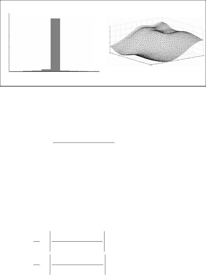
The results of identification of object (9) under noise conditions (10) are presented in Fig. 3. The figure presents the

noise histogram (Fig. 3a) and restored surface (Fig. 3b). After 2000 training epoches, the following estimates for noise

parameters were obtained:

05860= .

;

12 5818= .

;

00333= .

;

01646=- .

. The network consisted of 13 neurons

(seven neurons with BFs of the form (5) and six neurons with BFs of the form (6)).

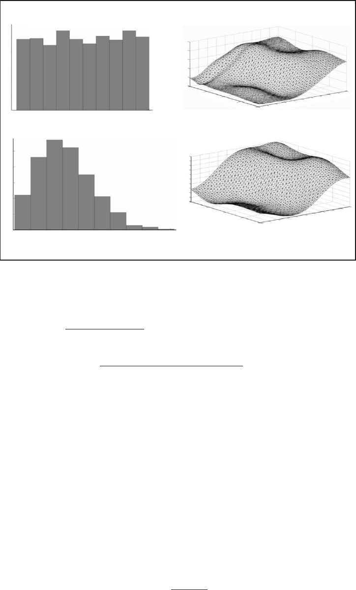
Experiment 2. The problem of identification of object (9) was considered in the presence of noise

x()k

uniformly

distributed according to the Rayleigh distribution (Ray (1.6)). In Figs. 4a and 4b, the noise histograms and forms of restored

surfaces, respectively, are presented.

Assuming that the real noise distribution is unknown, noise distributions in this experiment were approximated by

the Tukey–Huber model (10), which is used in [21, 22] and in which both the basic and contaminating distributions are

normal with estimates

0¹

. As a result of RBN training, the following contaminating noise parameters for the

uniform distribution were obtained:

=12.60

=1.83

, and

=-0.17

, and, for the Rayleigh distribution, the

parameters were as follows:

0 9981= .

08555= .

1 9702= .

, and

5 2842= .

; these estimates were used for

correcting output signals of the network. In this case, the network consisted of 14 neurons (five neurons with BFs of the

form (5) and nine neurons with BFs of the form (6)).

179

Fig. 3

–1

– 0.5

2500

2000

1500

1000

500

– 30 – 20 –10 0 10 20

Number of Noise Measurements

z in an Interval

Intervals

1.5

0.5

– 0.5

–1

0.5

– 0.4

0.4

yk()

yk()- 1

uk()- 1

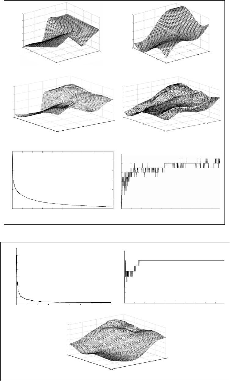
Experiment 3. The identification problem was solved for a multidimensional object (MIMO) described by the

following equations:

uk y k

15 1 1

250 1

05 1 0()

()()

[( )]

.( ).=

+--25 1 0 1

yk k(). ();-+ +x

uk yk uk

21 2

1121

()

(()()) ()

(),=

--+-

sin p

(12)

where

and

are input signals,

and

are output signals, and

and

are measurement noises.

The noise

was described by model (10) with the same parameters as in Experiment 1. The noise

has the

Rayleigh distribution (Ray (1.6)). Thus, the output signals of the object were subjected to different noises. Moreover, since

this object is multiconnected, the final kinds of distributions are very difficult to determine. After 2000 training epoches, the

following estimates for the noise parameters (for each separate output of the object) were obtained:

=1.2042

= 7.4612

00= .

, and

= 0.6765

for the first output and

= 2.5593

=1.5492

00= .

, and

= 2.0294

for the

second output.

The network consisted of 17 neurons (nine neurons with the BF whose number equals 1 and eight neurons with the

BF whose number equals 2 in Table 1). The simulation results are presented in Fig. 5. Figures 5a, 5b, 5c, and 5d present,

respectively, the reference surfaces described by expressions, restored surfaces, curve of changing the value of the fitness

function of the winner, and curve of changing the number of active neurons of the winner.

Experiment 4. Object (9) was identified with the same noise parameters as in Experiment 1 using the fitness-function

of the form (7) and the functional

specified by the expression

r[( )]

()

. (13)

Figures 6a and 6b present, respectively, the curve of changing the value of fitness-function (7) for the winner and the

curve of changing the number of active neurons. The restored surface is presented in Fig. 6c. The simulation results testify

that the use of fitness-function (7) with functional (13) allows one to efficiently eliminate noise using a simpler chromosome

format.

180

Fig. 4

–1

– 0.5

300

250

200

150

100

– 0,8 – 0,6 – 0,4 – 0,2 0 0,2 0 ,4 0,6

Number of Noise Measurements z

in an Interval

Intervals

1.5

0.5

– 0.5

–1

0.5

– 0.4

0.4

yk()

yk()- 1

uk()- 1

–1

– 0.5

600

500

400

300

200

100

012345

Intervals

0.8

0.6

0.4

0.2

– 0.2

– 0.4

– 0.6

– 0.8

–1

0.5

– 0.4

0.4

yk()- 1

uk()- 1

181

Fig. 5

–1

– 0.5

0.5

– 0.5

0.5

()

1()-

()

–1

– 0,5

Number

of Epochs

1.5

0.5

– 0.5

–1

–

– 1.5

0.5

– 0.5

0.5

()

1()-

()

1.5

0.5

– 0.5

–1

– 0,5

0,5

– 0,5

0,5

()

1()-

()

140

120

100

0 200 400 600 800 1000 1200 1400 1600 1800

0.5

– 0.5

–1

– 0.5

0.5

– 0.5

0.5

()

1()-

()

0 200 400 600 800 1000 1200 1400 1600 1800

0.5

– 0.5

–1

Fig. 6

23.5

22.5

21.5

20.5

19.5

0 100 200 300 400 500 600 700 800

Number

of Epochs

–1

– 0.5

0.5

– 0.5

0.5

yk()

yk()- 1

uk()- 1

0 100 200 300 400 500 600 700 800 900

–1

CONCLUSIONS

As is obvious from the simulation results, an evolving RBN using the GA for the specification of the structure of

a neural network-based model and estimation of its parameters has a high degree of robustness and is capable of solving the

identification problem for strongly noisy objects. Two approaches to the elimination of the influence of noise are possible in

this case. The first is based on the use of the Tukey–Huber model and consists of estimating noise parameters, and the

second approach is based on the use of M-training and allows one to somewhat simplify the structure of a chromosome since

it does not require any store for additional parameters. The simulation results demonstrate the efficiency of both approaches.

REFERENCES

1. I. J. Leontaritis and S. A. Billings, “Input-output parametric models for non-linear systems. Part I: Deterministic

non-linear systems,” Inf. J. of Control., 41, 303–308 (1985).

2. I. J. Leontaritis and S. A. Billings, “Input-output parametric models for non-linear systems. Part II: Stochastic

non-linear systems,” Int. J. of Control, 41, 309–344 (1985).

3. S. Chen and S. A. Billings, “Representations of nonlinear systems: The NARMAX model,” Int. J. of Control, 49(3),

1013–1032 (1983).

4. K. S. Narendra and K. Parthasarathy, “Identification and control of dynamical systems using neural networks,” IEEE

Trans. on Neural Networks, 1, No. 1, 4–26 (1990).

5. S. Chen, S. A. Billings, and P. M. Grant, “Recursive hybrid algorithm for non-linear system identification using radial

basis function networks,” Int. J. of Control., 55, 1051–1070 (1992).

6. S. Khaikin, Neural Networks: A Complete Course [in Russian], Izd. Dom “Williams,” Moscow (2006).

7. J. T. Spooner and K. M. Passino, “Decentralized adaptive control of nonlinear systems using radial basis neural

networks,” IEEE Trans. on Automatic Control, 44, No. 11, 2050–2057 (1999).

8. R. J. Shilling, J. J. Carroll, and A. F. Al-Ajlouni, “Approximation of nonlinear systems with radial basis function

neural networks,” IEEE Trans. on Neural Networks, 12, No. 6, 1–15 (2001).

9. O. G. Rudenko and A. A. Bessonov, “Real-time identification of nonlinear time-varying systems using radial basis

function network,” Cybernetics and Systems Analysis, 39, No. 6, 927–934 (2003).

10. Y. Li, N. Sundararajan, and P. Saratchandran, “Analysis of minimal radial basis function network algorithm for

real-time identification of nonlinear dynamic systems,” IEEE Proc., Control Theory Appl., 147, No. 4, 476–484 (2000).

11. D. L. Yu and D. W. Yu, “A new structure adaptation algorithm for RBF networks and its application,” Neural

Comput. & Appl., 16, 91–100 (2007).

12. E. P. Maillard and D. Gueriot, “RBF neural network, basis functions and genetic algorithm,” in: Proc. Int. Conf. on

Neural Networks, 4, Houston, TX (1997), pp. 2187–2192.

13. S. Ding, L. Xu, and H. Zhu, “Studies on optimization algorithms for some artificial neural networks based on genetic

algorithm (GA),” J. Computers, 6, No. 5, 939–946 (2011).

14. O. Buchtala, M. Klimek, and B. Sick, “Evolutionary optimization of radial basis function classifiers for data mining

applications,” IEEE Trans. on Systems, Man, and Cybernetics, Part B, 35, No. 5, 928–947 (2005).

15. P. Huber, Robustness in Statistics [Russian translation], Mir, Moscow (1984).

16. F. R. Hampel, E. M. Ronchetti, P. J. Rousseeuw, and W. A. Stahel, Robust Statistics: The approach Based on

Influence Functions, Wiley, N.Y. (1986).

17. D. S. Chen, and R. C. Jain, “A robust back-propagation learning algorithm for function approximation,” IEEE Trans.

on Neural Networks, 5, 467–479 (1994).

18. K. Liano, “A robust approach to supervised learning in neural network,” in: Proc. ICNN, 1 (1994), pp. 513–516.

19. Ch.-Ch. Lee, P.-Ch. Chung, J.-R. Tsai, and Ch.-I. Chang, “Robust radial basis function neural networks. Part B:

Cybernetics,” IEEE Trans. on Systems, Man, and Cybernetics, 29, No. 6, 674–685 (1999).

20. O. G. Rudenko and A. A. Bessonov, “Robust training of wavelet neural networks,” Probl. Upravl. Inf., No. 5, 66–79

(2010).

21. O. G. Rudenko and A. A. Bessonov, “Robust training of radial basis networks,” Cybernetics and Systems Analysis,

47, No. 6, 863–870 (2011).

22. O. Rudenko and O. Bezsonov, “Function approximation using robust radial basis function networks,” J. of Intelligent

Learning Systems and Appl., 3, 17–25 (2011).

23. O. G. Rudenko and A. A. Bessonov, “M-training of radial basis networks using asymmetric influence functions,”

Probl. Upravl. Inf., No. 1, 79–93 (2012).

182