EXTREME LEARNING MACHINE AND DEEP LEARNING NETWORKS

Hyperspectral image super-resolution using recursive densely

convolutional neural network with spatial constraint strategy

Jianwei Zhao

1,2

•

Taoye Huang

•

Zhenghua Zhou

Received: 29 January 2019 / Accepted: 29 August 2019

Ó Springer-Verlag London Ltd., part of Springer Nature 2019

Abstract

Hyperspectral images (HSIs) have been widely applied in real life, such as remote sensing, geological exploration, and so

on. Many deep networks have been proposed to raise the resolution of HSIs for their better applications. But training their

huge number of model parameters (weights and biases) needs more memory for storage and computation, which may bring

some difﬁculties when they are applied in mobile terminal devices. In order to condense the deep networks and still keep

the reconstruction effect, this paper proposes a compact deep network for HSI super-resolution (SR) by fusing the idea of

recursion, dense connection, and spatial constraint (SCT) strategy. We name this method as recursive densely convolu-

tional neural network with a spatial constraint strategy (SCT-RDCNN). The proposed method uses a novel designed

recursive densely convolutional neural network (RDCNN) to learn the mapping relation between the low-resolution (LR)

HSI and the high-resolution (HR) HSI and then adopts the SCT to improve the determined HR HSI. Compared with some

existing deep-network-based HSI SR methods, the proposed method can use much less parameters (weight and bias) to

attain or exceed the performance of methods with similar convolution layers because of the recursive structure and dense

connection. It is signiﬁcant and meaningful for the practical applications of the network in HSI SR due to the limitations of

hardware devices. Some experiments on three HSI databases illustrate that our propos ed SCT-RDCNN method outper-

forms several state-of-the-art HSI SR methods.

Keywords Hyperspectral image  Super-resolution  Deep convolutional network  Recursion  Dense connection

1 Introduction

A hyperspectral image (HSI) is a series of images that

record the spectrum of scene radiance by a distribution of

intensity in a contiguous band over a certain ele ctromag-

netic spectrum. As HSI contains the spectral signatures of

different objects, it has played a vital role in numerous

applications, such as geological exploration [1 ], face

recognition [2], object segmentation [3], and so on.

Although HSI can achieve high spectral resolution, it

has severe limitations in spatial resolution when compared

against regular RGB (a.k.a. multispectral) camera s in vis-

ible spectrum. The reason is that hyperspectral imaging

systems need a large number of exposures to acquire many

bands simultaneously within a n arrow spectral window.

While sensors obey a working princi ple that the wider the

visual ﬁeld is, the greater the cumulative energy reﬂects.

Therefore, whe n the spectral resolution is high, the spatial

resolution must be reduced to ensure enough energy for

imaging [4]. If people simply increase the resolution of the

imaging sensors, it will result in a lower signal-to-noise

ratio. The reason is that a less number of photons reach the

sensors [5]. Since super-resolution (SR) reconstruction

method acquires high-resolution (HR) image from one or a

series of low-resolution (LR) images by means of software

technique, it can enhance the spatial resolution without

compromising the existing devices. Therefore, people

& Jianwei Zhao

[email protected]

College of Sciences, China Jiliang University,

Hangzhou 310018, Zhejiang Province, People’s Republic of

China

State Key Laboratory for Novel Software Technology,

Nanjing University, Nanjing 210093, People’s Republic of

China

123

Neural Computing and Applications

https://doi.org/10.1007/s00521-019-04484-3

(0123456789().,-volV)(0123456789().,-volV)

begin to improve the spatial resolution of HSI by means of

SR reconstruction methods.

Up to now, many HSI SR methods have been proposed

to improve the resolutio n of HSIs. Some fusion methods

have been proposed for obtaining the HR HSI by com-

bining a LR HSI with a HR panchromatic image (covering

a large spectral window), such as linear transformations

(e.g., intensity-hue-saturation (IHS) transform [6], princi-

pal component analysis, wavelet transform [7–9]), unmix-

ing-based [10–12], and joint ﬁltering [13]. Those

approaches, originally developed by the community of

remote sensing, have been known as pansharpening and

especially suitable for the case where the spectral-resolu-

tion difference between two input images is relatively

small. With the development of sparse representation the-

ory [14], some sparsity-based methods have also been

proposed for HSI SR. Zhao et al. [15] proposed sparse

representation and spectral regularization algorithm that

uses the sparse prior to enhance the spatial resolution.

Simoes et al. [16] used a regularized form based on vector

total variation to fuse LR HSI wi th HR multispectral

images to get HR HSI. Dong et al. [17] proposed a non-

negative structure sparse representation model that trans-

forms the HSI SR into a joint estimate of spectral basis and

sparse coefﬁcients. However, most of these methods

tackled the HSI SR problem as an image fusion problem

using an auxiliary HR image. In the reality, it is very dif-

ﬁcult to obtain a couple of HR panchromatic image and

HSI about the same scene with completely registration,

which makes this kind of method not so practical.

Recently, as convol ution neural network (CNN) can

extract the high-level features and explore the contextual

information, it has been widely applied in man y computer

vision ﬁelds, such as face reco gnition [18], visual recog-

nition [19], natural image super-resolution [20], and so on.

In the last two years, CNN has also been applied in the HSI

SR. Yuan et al. [21] transferred the CNN with three con-

volution layers in [22] to learn the mapping relationship

between LR and HR HSI images. But this method did not

consider the spectral information preservation and the

difference between HSI and RGB images. For this, Li et al.

[5] p roposed an HSI SR method by combining a deep

spectral difference convolutional neural network (SDCNN)

with a spatial constraint (SCT) strategy, denoted by SCT-

SDCNN method. It still uses the CNN as in paper [21] with

three convolution layers but to learn the spectra l difference

mapping between the LR HSI and HR HSI . Furthermore, it

applies SCT strategy to constrain the LR HSI generat ed by

the reconstructed HR HSI spatially close to the original LR

HSI. Subsequently, people begin to consider constructing

more complex deep networks for HSI SR inspired the work

done for natural image SR. For example, He et al. [23]

proposed an HSI SR method inspired by a deep Laplacian

pyramid network to enhance the spatial resolution with the

spectral information preserved . Then, a nonnegative dic-

tionary learning method is proposed for spectral informa-

tion reconstruction. These deep-network-based HSI SR

methods have good reconstruction effect because of the

outstanding performance of deep networks. What is more,

these methods do not need the auxiliary panchromatic

image and multispectral image of the same scene.

Generally speaking, for given training data, before the

network is over-ﬁtted, the deeper the network is, the better

the reconstruction effect is. But increasing the depth of the

network will make the number of network parameters

(weight and bias) explode quickly. For example, even

highway network [24] with about 18 convolution layers for

the natural image SR, its number of parameters is about

1,000,000. Since HSI consists of many 2D images in dif-

ferent bands, which implies that HSI SR needs much more

model parameters than the natural image does. Therefore, it

will bring some troubles when it is applied in mobile ter-

minal devices. The reason is that when the depth of the

network increases, it needs not only more memory for

computation but also larger storage space. Of course, the

ordinary mobile terminal devices cannot satisfy the com-

puting requirement. Therefore, it is instructive to design a

deep network for HSI SR with less weights. Huang et al.

[25] proposed the idea of dense connection in DenseNet to

strengthen the feature propagation and encourage the fea-

ture reuse . It makes DenseNet use only a third of param-

eters in ResNet [

26] with the same effect. But DenseNet is

used to solve the classiﬁcation problem, not even for nat-

ural image SR.

In this paper, we want to propose a compact deep net-

work for HSI SR with less model parameters. We adopt the

idea of dense connection in DenseNet [25] to construct a

dense block for the deep network. But in order to further

reduce the network parameters in DenseNet while keeping

the approximate performance, we fuse the recursion idea

[27] on dense connection to design a more compact deep

network for HSI SR. We call the network recursive densely

connected neural network (RDCNN). The proposed

RDCNN uses the recursion to share the weights and biases

in the dense bloc k for reducing the number of model

parameters. Furthermore, with the SCT strategy, the

reconstructed HR HSI by RDCNN can be improved fur-

thermore. We name this HSI SR method as recursive

densely convolutional neural network with a spatial con-

straint strategy (SCT-RDCNN). The proposed SCT-

RDCNN can learn the mapping relation between the LR

HSI and HR HSI directly instead of the band difference in

SCT-SDCNN. The way of dense connection in our pro-

posed RDCNN can not only extract the high-level featur e

and allevi ate the problem of gradient vanishing and

exploding, but also use less weights than the network

Neural Computing and Applications

123

without dense connection. What is more, the recursive

operation in our RDCNN can use much less weights and

biases than the deep network with the same convolution

layers, while keeping the similar performance.

The main contributions of this paper are summarized as

follows:

1. This paper designs a compact deep network, named

SCT-RDCNN, for HSI SR by fusing the idea of

recursion, dense connection, and a spatial constraint

strategy.

2. Compared with the existing deep-network-based HSI

SR methods, the proposed RDCNN in SCT-RDCNN

can use much less parameters (weight and bias)

because of the recursive structure and dense connection

. It is signiﬁcant and meaningful for the practical

applications of the network in HSI SR due to the

limitations of hardware devi ces.

3. Experiments illustrate that the proposed SCT-RDCNN

can keep or exceed the accuracy of some state-of-the-

art deep networks for HSI SR with much less

parameters.

The remainder of this paper is organized as follows. Sec-

tion 2 describes the proposed SCT-RDCNN for HSI SR.

Section 3 carries out some comparison experiments of our

proposed SCT-RDCNN method with some other state- of-

the-art HSI SR methods. Lastly, the conclusions are given

in Sect. 4.

2 Proposed SCT-RDCNN for HSI SR

In this section, we give a description of the proposed SCT-

RDCNN for HSI SR in detail based on deep learning and

SCT strategy. The proposed SCT-RDCNN method designs

a novel RDCNN fusing the idea of recursion and dense

connection to get an HR HSI from the LR HSI and then

adopts the SCT strategy to further improve its reconstruc-

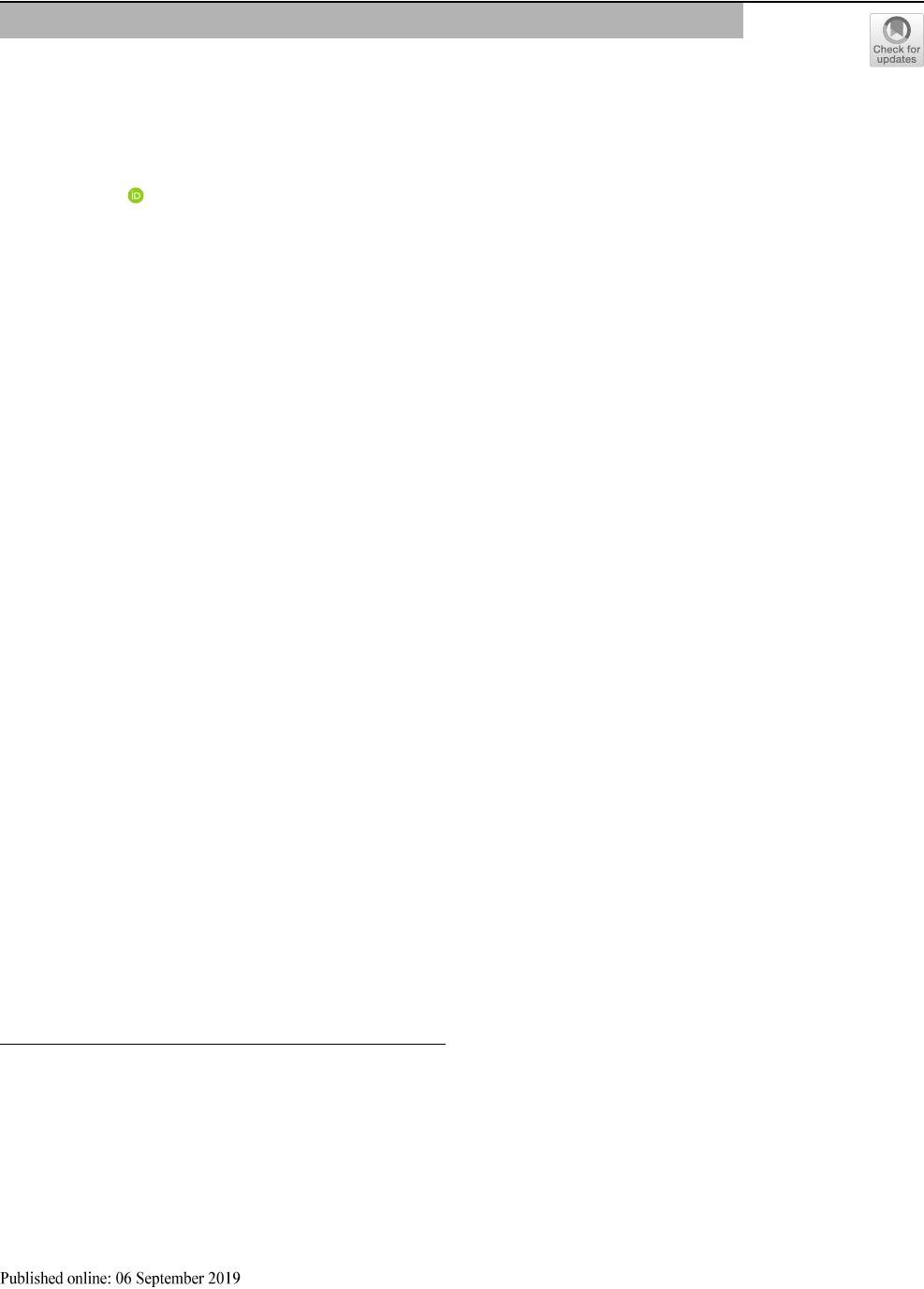
tion effect. The concrete structure diagram of our proposed

RDCNN is shown in Fig. 1, where RDCNN consists of

three main steps: initial feature extraction, recursive dense

block, and reconstruction. Figure 1a is the structure dia-

gram of our RDCNN with the folded form of the recursive,

and Fig. 1b is the corresponding structure diagram with the

unfolded form of the recursive with T times. In the fol-

lowing, we begin to explain the concrete process of our

SCT-RDCNN in detail.

2.1 Structure of RDCNN

In this subsection, we describe the structure of our pro-

posed RDCNN for HSI SR by fusing the recursion on

dense connection. In the process of designing the deep

network, we consider to reduce the model parameters

(weights and biases) by the idea of dense connection and

recursive operation. In the following, we explain the con-

crete structure of our RDCNN in three steps.

2.1.1 Initial Feature Extraction

The ﬁrst step of our proposed RDCNN is the initial feature

extraction. For the given LR HSI X 2 R

whb

, where w, h,

and b are the width, height, and bandwidth of X, respec-

tively, it is ﬁrstly magniﬁed r times with Bicubic. Here, we

note this up-sampled HSI as initial HR image

2 R

rwrhb

. Next we extract the feature map F

rwrhc

with the 3  3 convolution layer. Its process can

be d escribed in mathematics as:

¼ ReLUðW

 X

þ B

Þ; ð2:1Þ

where W

2 R

33bc

are weights with c channels, B

rwrhc

are the biases that have same elements in each

channel,  is the convolution operation as acting on the

RGB images, and ReLU is the operator that acts on each

element of matrices as

ReLUðxÞ¼maxf0; xg: ð2:2Þ

With the above initial feature extraction, we get an initial

HR HSI F

with low-level features.

2.1.2 Recursion with dense block

After getting the initial HR HSI F

, the next step is to

extract the high-level information by the proposed recur-

sive with dense block. As shown in Fig. 2, each dense

block in the proposed recursion contains mðm ¼ 4Þ basic

units and a transition unit, where the number m of basic

units can be chosen according to the appl ications. And each

basic unit consists of two convolution layers with different

kernels. The main structures of the proposed recursive

dense block are the dense connections in each dense block

and the recursive operation for the whole recursive model.

The step of dense connections in each dense block means

connecting the output of the early units to the later units,

which can make the network more compact and encourage

the features in different layers be reused fully. The step of

recursive operation means taking the output of the dense

block as the input of the dense block again, which makes

the dense block further extract the information by the same

weights and biases to save its storage space. Now we

explain the propos ed recursive dense block in two parts.

(1) Dense connection and units

In the block for recursive, we want to apply the idea of

dense connection in DenseNet [25] to improve the

Neural Computing and Applications

123

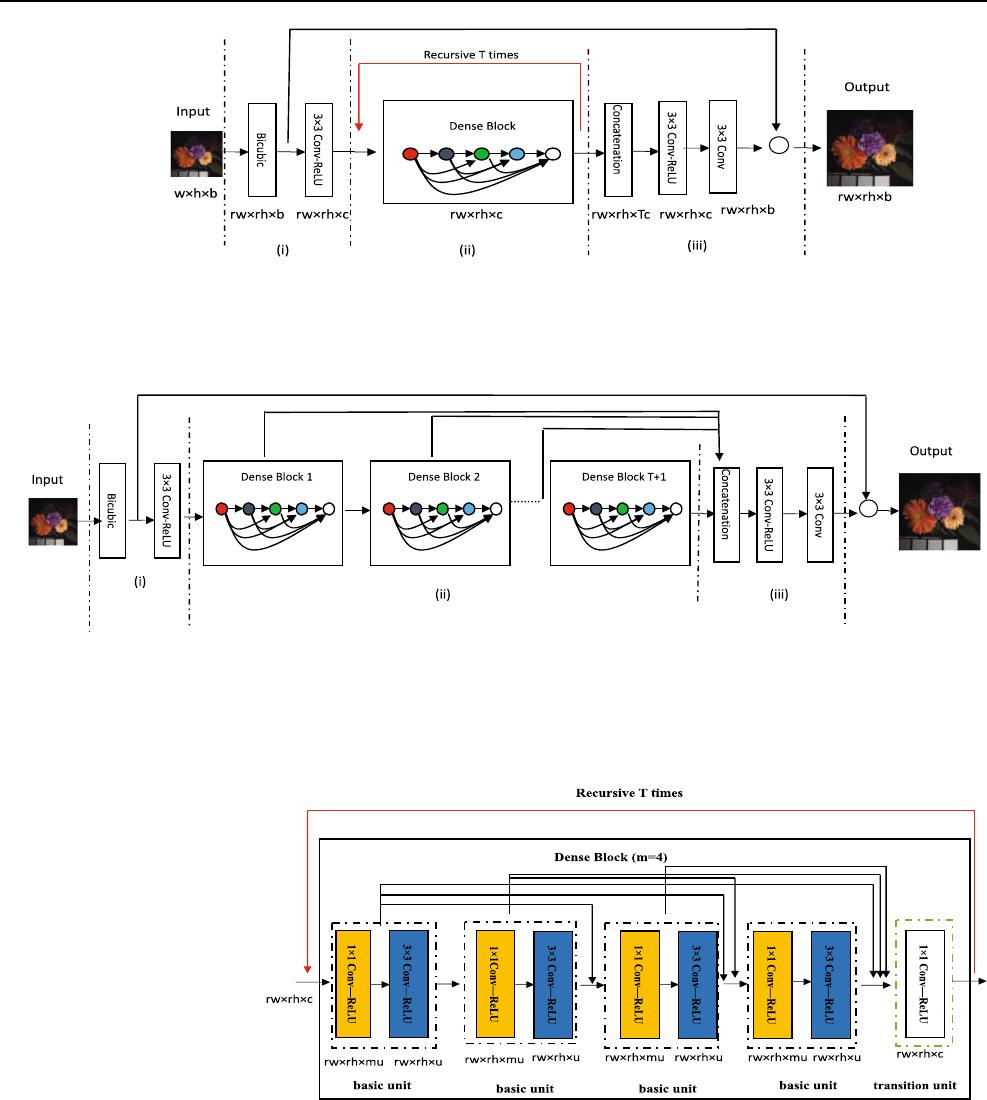
network’s performance. That is, we take some short con-

nections from the earlier units to the later units. Speciﬁ-

cally, the input of the latter basic unit composes all the

outputs of the earlier basic units, and its output will also be

sent to the latter basic units. This connection can not only

strengthen the feature propagation and encourage the fea-

ture reuse, but also use less weights than the network

without dense connection. For example, the dense

connection makes DenseNet use only a third of parameters

in ResNet [26] with the same effect.

With the dense connection, we begin to explain the

concrete structures of basic unit and transit unit in detail.

Generally speak ing, many deep networks use one type

convolution layer as a basic unit. However, in our proposed

network, we take two convolution layers with size of 1  1

and 3  3 as the basic unit. The reas on is that as the

(a) Structure diagram of our proposed RDCNN with the folded form of the recursive,

where the numbers under modules denote the size of feature maps after above

module operation. (i) Initial feature extraction. (ii) Recursive dense block. (iii)

Reconstruction.

(b) Structure diagram of our proposed RDCNN with the unfolded form of the recursive with T times. (i) Initial feature

extraction. (ii) Unfolded form of the recursive with T dense blocks. (iii) Reconstruction.

Fig. 1 The concrete structure diagram of our proposed RDCNN. a The folded form of the recursive. b The unfolded form of the recursive with

T dense blocks

Fig. 2 Internal architecture of

each dense block with mðm ¼

4Þ basic units and a transition

unit for the proposed recursive.

Two convolution layers (Conv-

ReLU) with different kernels in

a black dotted line rectangle

compose a basic unit. The last

convolution layer in a green

dotted line rectangle composes a

transition unit. The numbers

under modules denote the size

of feature maps after the above

module operation (colour

ﬁgure online)

Neural Computing and Applications

123

number of units increases, the number of channels in the

input will become large due to the dense connections.

Inspired by the idea in [25], we take a 1  1 convolution

layer before 3  3 convolution layer to reduce the number

of channels ﬁrstly for improving the computational efﬁ-

ciency. The output F

2 R

rwrhu

of the 1-st basic unit can

be represented as:

¼ ReLUðV

ðReLUðW

 Y þ B

ÞÞ þ D

Þ; ð2:3Þ

where Y 2 R

rwrhc

is the input of the dense block, W

11cmu

and V

2 R

33muu

are weights of 1  1 con-

volution layer and 3  3 convolution layer, respectively,

2 R

rwrhmu

and D

2 R

rwrhu

are biases of 1  1

convolution layer and 3  3 convolution layer, respec-

tively, and u is the number of output channels of each basic

unit.

The output F

2 R

rwrhu

of the jth basic unit in the

dense block has the similar expression as that for the 1-st

basic unit in (2.3) except the size of weights in the 1  1

convolution layer. For convenience, we just state the dif-

ference of the weights in the 1  1 convolution layer. That

is, W

2 R

11ðj1Þumu

because of the dense connection,

here W

is the weight of 1  1 convolution layer in the jth

basic unit, j ¼ 2; 3; ...; m.

In the end of dense block, a transition unit is designed to

guarantee the implementation of the recursion. As shown in

Fig. 2, if there is no transition unit, the output of m basic

units will be sent to the dense block again. However, its

number of channels u may not be same with the number of

channels c for the input of the dense block. In order to

guarantee the implementation of the recursive, a transition

unit is added at the end of block to compres s the number of

channels. The transition unit consists of one 1  1 convo-

lution layer whose weights W

mþ1

2 R

11muc

and biases

mþ1

2 R

rwrhc

. Its process can be described in mathe-

matics as:

mþ1

¼ ReLUðW

mþ1

½F

; F

; ...; F

þB

mþ1

Þ; ð2:4Þ

where ½F

; F

; ...; F

 is the concatenation of all the out-

puts of m basic units.

(2) Recursive operation

Generally, in order to achieve more effective perfor-

mance, people often deepen the network under a ﬁxed

width, which results in the explosion of the number of

weights. In order to reduce the number of weights and keep

a good performance of deep network, the idea of recursive

operation is utilized. As shown in Fig. 2, the output of

dense block is not only sent to the part of reconstruction,

but also sent back to the dense block again. It can also be

seen in the unfolded form of the recu rsive in Fig. 1b, where

we give T times that the feature map s have passed through

the dense block. With the recursive operation, we can

deepen the network by largening T, while not increasing

the number of weights and biases because of sharing the

same weights and biases in the dense block. Hence, it is not

like the traditional feedforward deep networks that use

different weights in different convolution layers to improve

the network’s performance. In the meanwhile, the higher-

level features can still be extracted by the deep structure

constructed by the recursive operation. When T ¼ 0, the

feature maps will be sent to the subsequent reconstruction

network directly. That is, it is the general feedforward

dense network.

The recursive operation can be inferred by the following

mathematical formula:

iþ1

¼RðK

Þ; ð2:5Þ

where K

iþ1

2 R

rwrhc

is the output of the dense block

after i times recursive operation, i ¼ 0; 1; 2; ...; T, and R is

the complex nonlinear function of the whole dense block

which is described in Sect. 2.1.2(1) in detail.

2.1.3 Reconstruction

As shown in Fig. 1b, in order to take ful l advantage of

different-level features produced by each recursion, we

concatenate them together to form the input of the recon-

struction part, where ‘‘concatenation’’ means the operation

that puts all the outputs of each recursion together. It is

noted that the input of the reconstruction part contains

high-level features because it passes through T recursion of

dense block.

The reconstruction part of our proposed RDCNN con-

sists of two convolution layers with size 3  3. The ﬁrst

3  3 convolution layer can fuse the feature information of

the input and sent out the feature maps with c channels for

the second convolution layer. The output X

2 R

rwrhb

the reconstruction part can be represented as:



V ðReLUð



W ½K

; K

; ...; K

Tþ1

þ



BÞÞ þ



ð2:6Þ

where ½K

; K

; ...; K

Tþ1

2R

rwrhðTþ1Þc

is the input of the

reconstruction part,



W 2 R

33ðTþ1Þcc

and



V 2 R

33cb

are weights of two convolution layers, respectively, and



B 2 R

rwrhc

and



D 2 R

rwrhb

are biases of two convo-

lution layers, respectively.

After the above two convolution operations, we get a

part of HR image that mainly contains the high-level fea-

ture information. Because the initial HR image X

magni-

ﬁed by Bicubic is full of the low-level information, we take

a skip connection from the initial HR image X

to the

output of the reconstruction part X

, which is also the

residual idea of ResNet [26]. Then, their sum, X

þ X

,as

Neural Computing and Applications

123

shown in Fig. 1b, is taken as the ﬁnal HR HSI

X. Owing to

the high correlation of low-level information and high-

level information, the skip connection can make the net-

work more effective.

2.2 Training

With a constructed RDCNN in Sect. 2.1, we begin to train

the network to determine the model parameters H ¼

; W

; ...; W

mþ1

; V

; ...; V

; B

; ...; B

mþ1

;

; D

; ...; D

;



Dg, where W

; W

; ...;

mþ1

; V

; ...; V

;



V are the weights in different con-

volution layer, and B

; B

; ...; B

mþ1

; D

; ...; D

;



are the biases in different convolution layer. In the training

process of RDCNN, values of these parameters are ini-

tialized from a Gaussian distribution with zero mean and

the variance is 0.001. The optimum values of these

parameters are achieved through minimizing the loss

between the reconstructed HR HSI RDCNNðX

Þ and the

corresponding HR HSI Y

; i ¼ 1; 2; ...; n. Mean squared

error (MSE) is utilized as the loss function:

LðHÞ¼

i¼1

kRDCNNðX

ÞY

;

ð2:7Þ

where fðX

; Y

Þg

i¼1

are the set of training samples. The loss

LðHÞ is minimized by stochastic gradient descent (SGD)

with the back- propagation [ 28 ].

2.3 Enhancement by SCT strategy

After reconstructing an HR HSI from the LR HSI with the

proposed RDCNN, we want to enhance its reconstruction

effect further with the SCT strategy in [5].

The idea of SCT strategy is that if the reconstructed HR

image

Z is close to the real one, its LR image with the same

degradation process will be clos e to the original LR image

X. Its objective function can be described as:

Z ¼ arg min

Z  G #X

;

ð2:8Þ

where Z is a reconstructed HR image, G is the blurry

kernel,  is the convolution operation, ‘‘#’’ is the down-

sampling operation, and X is the original LR HSI image.

Since the blur operation and downsampling operation

can be completely offset by the corresponding inverse

operation, the gradient descent for the above objective

function (2.8) is:

¼ 2 ðZ  GÞ#XðÞ"G;

ð2:9Þ

where ‘‘"’’ is the upsampling operation and  is the deblur

operation.

Take the reconstructed HR HSI with the RDCNN as the

initial value, i.e., Z

X, then the iterative formula for

(2.8) can be given as follows:

¼ Z

t1

 sððZ

t1

 GÞ#XÞ"G;

ð2:10Þ

where t denotes the number of iterations and s is the

learning step. Af ter q iterations, Z

is the ﬁnal recon-

structed HR HSI.

We name the HSI SR method that consists of RDCNN

and SCT strategy as SCT-RDCNN.

3 Experimental results

In this section, we will carry out some comparison exper-

iments on three benchmark datasets to demonstrate the

better performance of our proposed SCT-RDCNN than

some other state-of-the-art HSI SR methods.

All of our experiments are carried our in TensorFlow

1.6.0 version running in Intel

Xeon

E5-1620 v3 pro-

cessor with the speed of 3.50 GHz, four kernels, memory

of 32 GB, Windows 10.

3.1 Datasets

CAVE database [29] CAVE database contains many image

subdatabases for different tasks. Here, we select Mul-

tispectral Image Database for HSI super-resolution com-

parison experiments. This subdatabase consists of 32 scene

images containing a wide variety of real-world materials

and objects. The spatial size of all images is 512  512,

and the wavelength of images ranges from 400 to 700 nm

in a step of 10 nm (31 bands total).

Foster database [30] For the Foster database, we choose

the subdatabase: Hyperspectral Images of Natural Scenes

2002 for the comparison experiment. The subdatabase

contains 4 urban scenes from Porto and Braga and 4 rural

scenes from Minho in Portugal with different image size.

The wavelength of images ranges from 400 to 700 nm in a

step of 10 nm (31 bands total).

Harvard database [31] The Harvar d database provides

50 outdoor scenes and 27 indoor scenes HSIs. The spatial

size of these images is 1040  1392, and the wavelength of

images ranges from 420 to 720 nm in a step of 10 nm (31

bands total).

In this paper, we choose two HSI images from each

datasets for the testing and the remaining images for the

training as mentioned in [5]. In order to provide an eye-

appealing exhibition about the HSI, we create a RGB

image for each HSI by averaging the 1-st band to the 11-th

band as the B channel, the 11-th band to the 21-st band as

the G channel, and the 21-st band to the 31-st band as the

Neural Computing and Applications

123

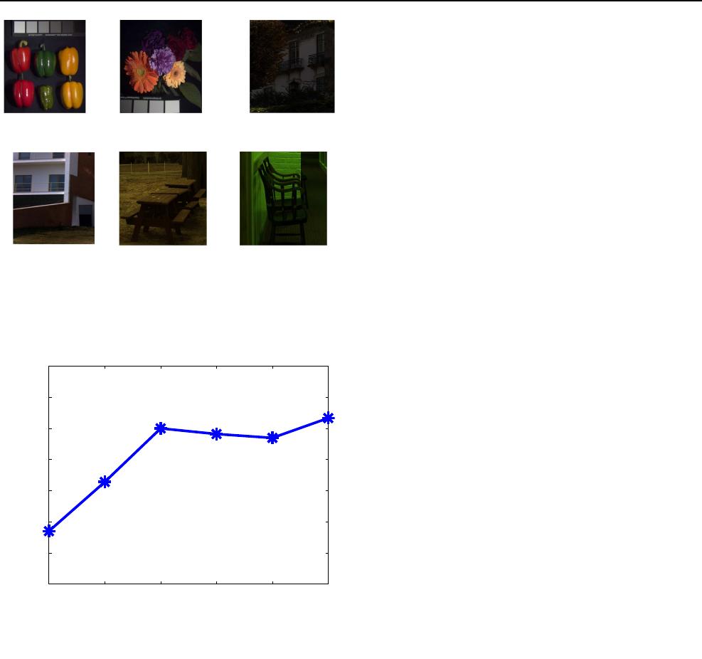
R channel. Then, the corresponding RGB images for the

selected testing HSIs are shown in Fig. 3.

For constructing the training images for our networks,

we take the selected HSIs from databases as the HR ima-

ges, and the corresponding LR images are generated by the

following degenerative process: (1) blur with Gaussian

ﬁlter; (2) down-sample with the scaling factor; (3) add

zero-mean Gaussian noise. Before inputting the LR images

into the network, in order to avoid the inﬂuence of different

ranges of data values, and improve the training speed of the

networks, both the LR and HR images are normalized.

3.2 Evaluation of RDCNN

The key points in our proposed RDCNN are the recursive

structure and dense connection, which is different from

most deep-network-based HSI SR methods. In this sub-

section, we want to carry out some comparison experi-

ments on RDCNN to explain the signiﬁcance of these

structures. In the meanwhile, our RDCNN has several key

parameters related to the network structure and perfor-

mance: the recursive time T, the number of basic units m in

a dense recursive block, the number of output channels u of

each basic unit, and the number of output channels c of the

initial feature maps in F

or transit unit. Therefore, we

design some experiments on these parameters to show the

performances of our propos ed RDCNN.

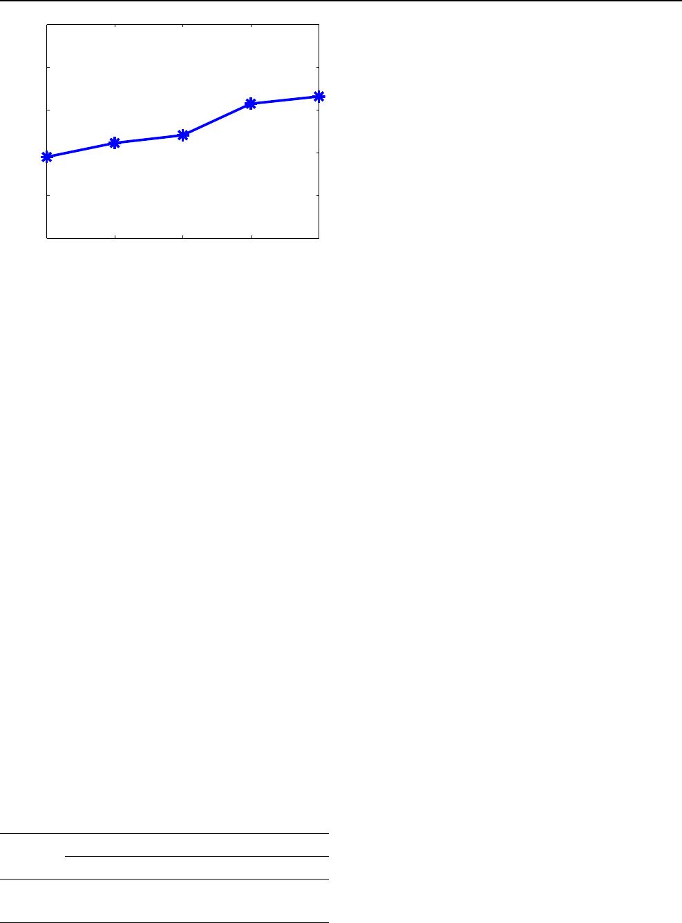
3.2.1 Impact of the recursive time T

In this experiment, we wan t to illustrate the impact of the

recursive times T on the performance of our proposed

RDCNN. The other parameters are taken as follows: the

number of basic units in a dense recursive block m ¼ 5, the

number of output channels of the basic unit u ¼ 12, and the

number of output channels of the transit unit c ¼ 12 by

experience. Then, the average peak signal-to-noise ratio

(PSNR) (dB) of the reconstructed HSI by RDCNN on 6

testing images varying with the recursive time T is shown

in Fig. 4.

As observed from Fig. 4, when T increases from 1 to 3,

the average PSNR of 6 testing images also increases. But

when T is greater than 3, average PSNR began to ﬂuctuate.

The reason is that the size of T is equivalent to the depth of

the network. The reason is that when T increases, the

network is deepened. Generally, the deepening of network

will improve the network’s learning ability. Therefore, the

average PSNR will increase from T = 1 to 3. But dense

blocks in our RDCNN share the common weights and

biases to extract the features, so it is impossible to increase

learning ability inﬁnitely. Since the aver age PSNR of the 6

testing images is basically same when T starts from 3, we

determine T ¼ 3 considering the minimum amount of

calculation.

3.2.2 Impact of the number of basic units

In this experiment, we wan t to illustrate the impact of the

number of basic units m in the dense block in our RDCNN.

Here, we take the recursive times T ¼ 3, u ¼ 12, and c ¼

12 as explained in Sect. 3.2.1. Then, the average PSNR

(dB) of the reconstructed HSIs by RDCNN on 6 testing

images varying with the number of basic units m is shown

in Fig. 5.

(a) Peppers (b) Flowers (c) Scenes6

(d) Scenes7 (e) Imgb0 (f) Imgg1

Fig. 3 The RGB images for the selected testing HSIs from three

different databases. a Flowers and b Peppers from CAVE database,

c Scenes6 and d Scenes7 from Foster database, and e Imgb0 and

f imgg1 from Harvard database

1 2 3 4 5 6

41.5

41.6

41.7

41.8

41.9

42.1

42.2

Recursive Times

Average PSNR of test images(dB)

Fig. 4 The average PSNR (dB) of the reconstructed HSIs by RDCNN

on 6 testing images varying with the recursive time T

Neural Computing and Applications

123

As observed from Fig. 5, the average PSNR of the

reconstructed HSIs increases when the number of basic

units m increases. Generally, both m and T are considered

as the parameters that determ ine the depth of the network.

The difference between m and T is that increment of m is

equivalent to adding convolution layers with different

weights. Since the total number of convolution layers in

our RDCNN is not very large, the learning ability of net-

work will continue to increase as the depth increases. That

is, the average PSNR in Fig. 5 for the reconstructed HSIs

will go up. A larger m may result in a better result, but

considering the cost of computation, we take m ¼ 9 in the

subsequent experiments.

3.2.3 Impact of the number of channels u and c

In this experiment, we wan t to illustrate the impact of the

number of the output channels u of the basic unit and the

number of output channels c of the initial feature maps or

transit unit in the dense block in our RDCNN. Here, we

take the recursive times T ¼ 3 and the number of basic

units m ¼ 9 as explained in Sects. 3.2.1 and 3.2.2,

respectively. Table 1 shows the average PSNR of our

proposed RDCNN on 6 testing images with varying u and

As shown in Table 1, with the ﬁxed number of the

output channels u of the basic unit, when the number of

output channels c of the initial feature maps or transit unit

increases, the average PSNR (dB) of the reco nstructed

HSIs by RDCNN on 6 testing images increases ﬁrstly and

then ﬂuctuates. With the ﬁxed number of output channels c

of the initial feature maps or transit unit, except the case

c ¼ 12, when the number of the output channels u of the

basic unit is larger, the average PSNR (dB) of the recon-

structed HSIs by RDCNN on 6 testing images becomes

better. Generally, both u and c are related to the width of

the network. When the numbers of channels u and c

increase, the network performance will be improved

because of the widened network structure. Fo r the case

c ¼ 12, the performance of our RDCNN becomes worse.

The reason is that the information extracted by the initial

feature extraction is not rich enough, and it is difﬁcult to

support the recursive dense block with stronger learning

ability to further extract features. Therefore, u and

c need a

suitable combination. Considering the number of weights

and biases and the effect of our network, we choose u ¼ 24

and c ¼ 24.

3.3 Reconstruction comparison of our method

with others

In this subsection, we compare our proposed RDCNN and

SCT-RDCNN with some other HSI SR methods: Bicubic,

SNNMF [32], CNMF [33], HySure [16], NSSR [17], and

SCT-SDCNN [5]. We take the root mean square error

(RMSE), structural similarity (SSIM), and PSNR as the

evaluation criterion. For the methods that require the

auxiliary image (e.g., multispectral images) to assist the

reconstruction, we utilize the approach of generating RGB

images in Sect. 3.1 as the alternative. The comparison

results of the average PSNR, RMSE, and SSIM of our

proposed RDCNN, SCT-RDCNN, and some other HSI SR

methods under different magniﬁcation times r on the

reconstructed 6 HSIs are shown in Table 2.

As observed from Table 2, our proposed RDCNN, SCT-

RDCNN methods and SCT-SDCNN [5] have better per-

formances than the other HSI SR methods. The reason is

that our proposed RDCNN, SCT-RDCNN methods and

SCT-SDCNN [5] are based on deep networks that have

strong feature representation ability. What is more, our

proposed RDCNN performs better than SCT-SDCNN [5]

except the case r ¼ 3, where the PSNR and RMSE are

worse than those of SCT-SDCNN [5]. The reason is that

the SCT strategy acts an important role in the reconstruc-

tion results when the magniﬁcation times r is not large.

However, when we also adopt the SCT strategy on our

5 6 7 8 9

41.8

41.9

42.1

42.2

42.3

The number of basic unit in recursive dense block

Average PSNR of test images(dB)

Fig. 5 The average PSNR (dB) of the reconstructed HSIs by RDCNN

on 6 testing images varying with the number of basic units m in a

recursive dense block

Table 1 The average PSNR (dB) of our proposed RDCNN on 6

testing images with varying number of the output channels u of the

basic unit and the number of output channels c of the initial feature

maps or transit unit

12 24 36 48

12 42.11 42.15 42.19 41.92

24 37.21 42.31 42.31 42.29

Neural Computing and Applications

123

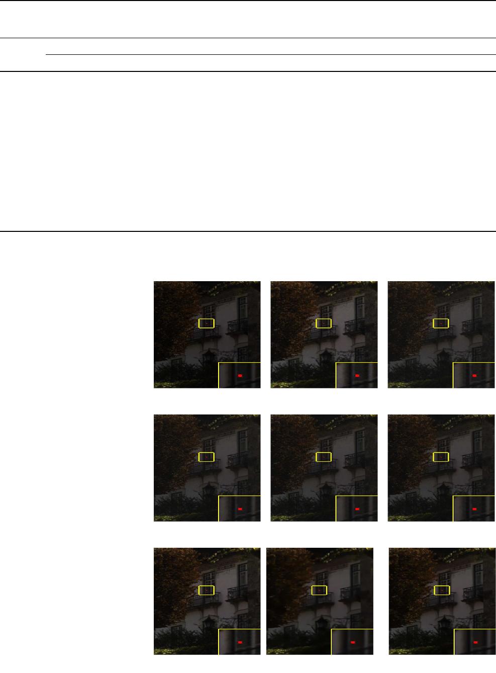
(a) Original (b) Bicubic (c) SNNMF

(d) CNMF (e) HySure (f) NSSR

(g) SCT-SDCNN (h) RDCNN (i) SCT-RDCNN

Fig. 6 Visual comparison of

reconstructed high-resolution

hyperspectral images for

‘‘scene6’’ image with different

methods

Table 2 Comparison of the average PSNR, RMSE, and SSIM of the reconstructed HSIs on 6 images by our proposed RDCNN, SCT-RDCNN,

and some other HSI super-resolution methods under different scales

Scales Methods

Bicubic SNNMF [32] CNMF [33] HySure [16] NSSR [17] SCT-SDCNN [5] RDCNN SCT-RDCNN

PSNR 37.19 36.95 37.62 37.97 38.02 41.03 42.33 44.30

RMSE 0.0140 0.0143 0.0132 0.0127 0.0126 0.0092 0.0082 0.0064

SSIM 0.8267 0.8752 0.8838 0.8979 0.9011 0.9192 0.9597 0.9827

PSNR 35.48 36.32 36.54 36.97 37.03 39.15 39.05 41.30

RMSE 0.0172 0.0151 0.0143 0.0129 0.0125 0.0117 0.0118 0.0091

SSIM 0.8184 0.8225 0.8530 0.8889 0.8861 0.9040 0.9375 0.9673

PSNR 35.43 35.39 36.32 36.75 36.79 37.97 38.46 40.17

RMSE 0.0174 0.0170 0.0153 0.0145 0.0145 0.0131 0.0128 0.0105

SSIM 0.8173 0.8112 0.8379 0.8573 0.8586 0.8992 0.9267 0.9557

Neural Computing and Applications

123

RDCNN, our proposed SCT-RDCNN can improve almost

2 on PSNR, 0.03 on SSIM, and 0.002 on RMSE than our

RDCNN does. Then, the PSNR and RMSE of our proposed

SCT-RDCNN are better than those of SCT-SDCNN [5]. In

summary, our proposed SCT-RDCNN outperforms better

than all the HSI SR methods in Table 2.

In order to give a visual feel of those HSI SR methods in

Table 2, we exhibit the reconstruction image of the image

‘‘scene6’’ from Harvard database in Fig. 6. Furthermore,

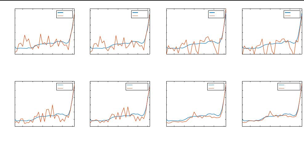
the spectral curves of the red pixel by different recon-

struction methods in Fig. 6 are shown in Fig. 7.

As observed from the local enlarged patches in Fig. 6,

our proposed SCT-RDCNN can reconstruct the HR HSI

closer to the original HSI than the other methods. In the

meanwhile, Fig. 7 shows that the spectral curves of the red

pixel reconstructed by our RDC NN and SCT-RDCNN are

closer to the curve of the red pixel in the original HSI than

other methods do.

4 Conclusion

In this paper , an efﬁcient hyperspectral image (HSI) super-

resolution method has been proposed based on a proposed

recursive densely convolutional neural network (RDCNN)

and the spatial constraint (SCT) strategy, denoted by SCT-

RDCNN method. The proposed RDCNN that fuses the idea

of dense connection and recursion is designed to learn the

mapping relation between the low-resolution (LR) HSI and

the high-resolution (HR) HSI directly. The way of dense

connection in our proposed RDCNN can not only extract

the high-level feature and alleviate the problem of gradient

vanishing and exploding, but also use less weights than the

network without dense connection. In the meanwhile, the

recursive operation in our RDCN N can use muc h less

weights and biases than the deep network with the same

convolution layers because of the shared weights and bia-

ses, while keeping the similar performance. Based on the

good performance of RDCNN, the spatial constraint (SCT)

strategy is used to enhance the effect of reconstructed HR

HSI. Some experiments on three databases illustrate that

our proposed SCT-RDCNN method outperforms several

state-of-the-art HSI SR methods.

Acknowledgements This work was funded by the National Natural

Science Foundation of China (61571410) and the Zhejiang Provincial

Nature Science Foundation of China (LY18F020018 and

LSY19F020001).

Compliance with ethical standards

Conflict of interest The authors declare that they have no conflict of

interest.

Research involving human participants and/or animals This study did

not involve human participants and animals.

Informed consent The all authors of this paper have consented to the

submission.

References

1. Asadzadeh S, de Souza CR (2016) A review on spectral pro-

cessing methods for geological remote sensing. Int J Appl Earth

Obs Geoinform 47:69–90

5 1015202530

band number

0.02

0.04

0.06

0.08

0.1

0.12

value

original

bicubic

(a) Bicubic

5 1015202530

band number

0.02

0.04

0.06

0.08

0.1

0.12

value

original

SNNMF

(b) SNNMF

5 1015202530

band number

0.02

0.04

0.06

0.08

0.1

0.12

value

original

CNMF

5 1015202530

band number

0.02

0.04

0.06

0.08

0.1

0.12

value

original

HySure

(d) HySure

5 1015202530

band number

0.02

0.04

0.06

0.08

0.1

0.12

value

original

NSSR

(e) NNSR

5 1015202530

band number

0.02

0.04

0.06

0.08

0.1

0.12

value

original

SCT_SDCNN

(f) SCT-SDCNN

5 1015202530

band number

0.02

0.04

0.06

0.08

0.1

0.12

value

original

RDCNN

(g) Our RDCNN

5 1015202530

band number

0.02

0.04

0.06

0.08

0.1

0.12

value

original

SCT_RDCNN

(h) Our SCT-RDCNN

Fig. 7 Comparison of the spectral curves of the red pixel in Fig. 6 reconstructed by different methods

Neural Computing and Applications

123