
Optimization Letters
https://doi.org/10.1007/s11590-020-01643-7
ORIGINAL PAPER
Iterated local search for the generalized independent set
problem
Bruno Nogueira
1
· Rian G. S. Pinheiro
1
· Eduardo Tavares
2
Received: 15 November 2019 / Accepted: 2 September 2020
© Springer-Verlag GmbH Germany, part of Springer Nature 2020
Abstract
The generalized independent set problem (GISP) can be conceived as a relaxation
of the maximum weight independent set problem. GISP has a number of practical
applications, such as forest harvesting and handling geographic uncertainty in spatial
information. This work presents an iterated local search (ILS) heuristic for solving
GISP. The proposed heuristic relies on two new neighborhood structures, which are
explored using a variable neighborhood descent procedure. Experimental results on
a well-known GISP benchmark indicate our proposal outperforms the best existing
heuristic for the problem. In particular, our ILS approach was able to find all known
optimal solutions and to present new improved best solutions.
Keywords Combinatorial optimization · Maximum independent set · Iterated local
search · Variable neighborhood descent · Metaheuristics
1 Introduction
Consider an undirected graph G = (V , E ), a subset of removable edges E
⊆ E,
revenues b(v
i
) for each vertex v
i
∈ V , and costs c(v
i
,v
j
) for each removable edge
(v
i
,v
j
) ∈ E
. The generalized independent set problem (GISP) aims at determining
an independent set S ⊆ V (i.e., a subset of vertices such that no two vertices are
adjacent) that maximize the profit, defined as the difference between selected vertex
B
Bruno Nogueira
Rian G. S. Pinheiro
Eduardo Tavares
1
Universidade Federal de Alagoas, Instituto de Computacão, Maceió, Brazil
2
Universidade Federal de Pernambuco, Centro de Informática, Recife, Brazil
123

B. Nogueira et al.
v
2
v
3
v
6
v
8
v
1
v
4
v
5
v
7
Fig. 1 The generalized independent set problem: instance and candidate solution
revenues and the total cost of deleting removable edges connecting them. GISP can
be conceived as a relaxation of the well-known maximum weight independent set
(MWIS) problem [1], i.e., it allows adjacent vertices to be in the independent set but
take into account the penalties of doing so. Due to this property, the GISP model has
potential to be applied to many practical applications, such as: forest harvesting [2],
handling geographic uncertainty in spatial information [3], facility location [4], and
cartographic label placement [5].
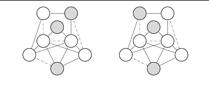
Figure 1 shows an instance of the GISP, and a candidate solution. Dashed edges
indicate the set of removable edges E
and gray vertices the set of solution vertices S.
The profit of this solution is calculated as: b(v
2
) + b(v
3
) + b(v
6
) + b(v
8
) − c(v
2
,v
6
).
GISP is computationally challenging since it belongs to the class of NP-hard
problems. As a consequence, current exact methods [2,6,7] for the problem are effi-
cient only on instances of limited sizes or instances with particular structures. In this
work, we focus on heuristic methods that seek high-quality sub-optimal solutions
in reasonable time. In [8], Kochenberger et al. modeled GISP as an unconstrained
binary quadratic problem (UBQP) and used a tabu search heuristic for it. Colombi
et al. [6] also casted the GISP as an UBQP and proposed a hybrid GRASP-tabu
search. The work of Colombi et al. further suggested two Linear Programming-based
heuristics, but their experimental results show that the GRASP-tabu search approach
outperforms them. Recently, Hosseinian and Butenko [7] proposed a construction
heuristic based on the optimization of a quadratic function over a hypersphere. To
the best of our knowledge, these are the only heuristic approaches for the GISP.
This situation contrasts with the great amount of heuristics for conventional inde-
pendent set problems [1,9] and other related problems, such as clique problems
[10,11].
In this work, we extend our recently proposed iterated local search (ILS) heuristic
[1], which was originally presented in the context of the MWIS, to the GISP. The
proposed heuristic relies on two new neighborhood structures that are explored using
a variable neighborhood descent (VND) procedure. Experimental results on a well-
known GISP benchmark indicate our proposal outperforms the best existing heuristic
for the problem. In particular, our ILS approach was able to find all known optimal
solutions and to present new improved best solutions.
123
ILS for the generalized independent set problem
v
1
v
6
v
8
v
2
v
3
v
4
v
5
v
7
(a) Neighborhood N
1
: resulting so-
lution after move N
1
(v
1
)
v
1
v
7
v
8
v
2
v
3
v
6
v
4
v
5
(b) Neighborhood N
2
: resulting so-
lution after move N
2
(v
1
,v
7
)
Fig. 2 Neighborhood structures
2 Neighborhood structures
This section describes the two proposed neighborhood structures for the problem: N
1
and N
2
, which consist in adding one and two vertices to the solution, respectively.
These neighborhoods are generated considering a solution with no free vertices, i.e.,
a solution in which a new vertex can only be added if at least one removable edge is
deleted or one vertex is removed from the solution.
An example of N
1
is illustrated in Fig. 2a, in which the original solution S (Fig. 1)
is modified by applying move N
1
(v
1
). This move inserts v
1
to the solution, but before
inserting it, the move either removes solution vertices that are adjacent to v
1
or deletes
removable edges between v
1
and the solution vertices. Whenever we have the option
of removing a vertex or deleting an edge, we choose the less costly option. Note
that, in this example, vertex v
3
does not remains in the solution, which implies that
b(v
3
)<c(v
1
,v
3
), i.e., the cost of deleting edge (v
1
,v
3
) is greater than the cost of
removing v
3
. An example of N
2
is depicted in Fig. 2b, which shows the resulting
solution after applying move N
2
(v
1
,v
7
) to S.
In the following, we describe the proposed procedures to find a move with positive
gain in these neighborhoods, i.e., a move that improves the current solution profit. We
remark that the proposed exploration procedures are not exhaustive, in the sense they
do not guarantee that an improving move will be found if such a move exits. However,
as the experimental results show, they offer a good balance between solution quality
and CPU time.
2.1 Data structures
To rapidly evaluate the gain of each candidate move in the considered neighborhoods,
our algorithm maintains four data structures (arrays with |V | elements) during the
search:
– tightness[v], which stores the number of vertices in the current solution that are
adjacent to v: tightness[v]=|{x ∈ S : (x,v)∈ E }|.
123

B. Nogueira et al.
– tightness
[v], which represents the number of solution vertices that are adjacent
to v through removable edges: tightness
[v]=|{x ∈ S : (x,v) ∈ E
}|.
– μ[v], which gives a lower bound on the gain of adding v to the solution, i.e., the
gain of adding v, and removing from the solution each adjacent vertex of v or
deleting the corresponding removable edges between v and the solution vertices:
μ[v]=b(v)−
x∈S
min(c
•
(x,v),b(x)), where c
•
(x,v)= c(x,v)if (x,v) ∈ E
,
and c
•
(x,v)=∞otherwise.
– μ
[v], which indicates the gain of removing v from the solution, i.e., the gain of
removing v and adding back the removable edges that were deleted when v entered
in the solution: μ
[v]=−b(v) +
x∈S
c
◦
(x,v), where c
◦
(x,v) = c(x,v) if
(x,v)∈ E
, and c
(x,v)= 0 otherwise.
Note that the value maintained in μ[v] is a lower bound on the gain of adding v
because this data structure does not take into account the possible gains of adding back
deleted edges. For instance, the gain of adding v
1
to the solution depicted in Fig. 1
would be b(v
1
) − min(b (v
3
), c(v
1
,v
3
)) − b(v
2
) + c(v
2
,v
6
). However, μ[v
1
] in this
case would be b(v
1
) − min(b(v
3
), c(v
1
,v
3
)) − b(v
2
). We store in μ a lower bound
instead of the exact value because computing t he exact gain would mean increasing
the complexity of adding/removing a vertex to/from the solution. Such a complexity
increase would eliminate all the benefit of maintaining data structure μ.
When our algorithm begins, these data structures have the following initial values for
each v ∈ V : tightness[v]=0, tightness
[v]=0, μ[v]=b(v), and μ
[v]=−b(v).
Algorithm 1 describes how they are updated whenever we add a new vertex to the
current solution. Such an add operation takes O(), where is the maximum graph
degree. In line 2 of Algorithm 1, we loop through each vertex y adjacent to the vertex
being added v. If condition at line 3 holds true, we assume that the edge (y,v) ∈ E
has been deleted (otherwise, the solution would become infeasible), thus tightness[v]
and tightness
[v] are decreased by one, and μ
[v] and μ
[y] are increased by c(y,v).
If condition at line 3 is false, tightness[y] is increased by one, and if additionally
(y,v)∈ E
, tightness
[y] is also increased by one. Note that, at the end of the loop,
the value of μ[y] for each y adjacent to v is decreased by b(v) if (y,v) /∈ E
, and by
min(b(v), c(y,v)), otherwise.
The procedure for updating the data structures when a vertex is removed is similar to
Algorithm 1. Except that at lines 4–8, 12, 13, and 15, subtract operations are exchanged
by sum operations and vice versa.
2.2 Neighborhood exploration
To find an improving move in N
1
, we propose two exploration procedures. The first
one takes O(|V |) and it works by searching for a vertex v ∈ V \ S, s uch that μ[v] >
0. If such a vertex is found, a N
1
(v) move will improve the solution. The second
exploration procedure is O(|E|). It consists in exploring each adjacent vertex of a
solution vertex x ∈ S and trying to find a vertex y ∈ V \ S, such that (x, y) ∈ E \ E
,
μ[y]+μ
[x]+b(x)>0. Applying a N
1
move to add such a vertex y also improves
the solution. The expression μ[y]+μ
[x]+b(x) gives the gain of adding y to the
123

ILS for the generalized independent set problem
Input : Vertex to be added v ∈ V , current solution S, input graph G = (V , E , b, c), data structures
tigthness, tigthness
, μ, μ
1 AddVertex(v, S, G, t ightness, ti ghtness
, μ, μ
)
2 foreach y ∈ Adj(v, G) do
3 if y ∈ S then // if true, then (y,v) ∈ E
and assume (y,v) was
removed
4 tightness[v]=tightness[v]−1
5 tightness
[v]=tightness
[v]−1
6 μ[y]=μ[y]−min(c((y,v)), b(v))
7 μ
[v]=μ
[v]+c((y,v))
8 μ
[y]=μ
[y]+c((y,v))
9 else
10 tightness[y]=tightness[y]+1
11 if (y,v)∈ E
then
12 tightness
[y]=tightness
[y]+1
13 μ[y]=μ[y]−min(c((y,v)), b(v))
14 else
15 μ[y]=μ[y]−b(v)
16 S = S ∪{v}
Algorithm 1: Pseudo-code for adding a vertex to the solution and updating data
structures tigthness, tigthness
, μ, and μ
.
solution, μ[y], plus the gain of adding back the removable edges that were deleted
when x entered in the solution, μ
[x]+b(x).
To find an improving move in neighborhood N
2
, we adapt the exploration procedure
for adding two vertices described in [9], which takes O(|E|). Such a procedure was
originally proposed in the context of the maximum independent set problem [9], and
its objective is to replace some vertex x in the solution with two vertices, u and v
(both originally outside the solution), thus increasing the total number of vertices in
the independent set by one.
Our adaptation has only two differences compared to the original procedure in [9].
The first difference is that in order to construct the list L(x) of 1-tight neighbors of
x ∈ S , we consider all vertices y ∈ V \ S, such that tightness[y]−tightness
[y]=
1,(x, y) ∈ E \ E
. The second difference is that, after finding two vertices u,v ∈
L(x), (u,v) /∈ E, we use the following condition to check if the solution will be
improved by adding u and v: μ[u]+μ[v]+μ
[x]+2b(x )>0. Note that other
vertices than x mayberemovedbyaN
2
(u,v)move. The expression μ[u]+μ[v]+
μ
[x]+2b(x ) denotes the gain of adding u and v, μ[u]+μ[v]+b(x), plus the gain
of adding back the removable edges that were deleted when x entered in the solution,
μ
[x]+b(x).
3 Proposed algorithm
ILS is a metaheuristic that explores the space of local optima in order to find a global
optimum [12]. It works as follows: first, the current local optimum solution is per-
turbed (changed). Then, local search is applied to the perturbed solution. Finally, if
123

B. Nogueira et al.
the solution obtained after the local search satisfies some conditions, it is accepted
as the new current solution. This process repeats until a given stopping criterion is
met. In this work, we use a VND based approach in the local search phase of the ILS
algorithm. The basic idea of VND is to successively explore a set of pre-defined neigh-
borhoods to improve the current solution [13]. Algorithm 2 describes the proposed
heuristic algorithm, called ILS-VND, for the GISP. It follows the same structure as
the algorithm presented in [1], by iteratively applying local search and perturbation
moves (lines 8 and 9), and then deciding the new current solution (line 10) by means
of some acceptance criteria.
Input : Input graph G = (V , E , b, c)
1 ILS-VND(G)
2 S
0
= Initialize(G) // initial solution
3 S = LocalSearch(S
0
,G) // current solution
4 S
∗
= S // best solution
5 local_best_ p = Profit(S) // best local profit
6 i =1 // local iteration counter
7 while stop criteria do
// perturb the current solution
8 S
= Perturb(c
1
,S,G)
// apply local search to the perturbed solution, using a VND
approach
9 S
= LocalSearch(S
,G)
// define the new current solution S, and update S
∗
, k,
local_best_ p
10 (S, S
∗
, i , local_best_ p)=Accept(S, S
∗
,S
,i,local_best_p,G)
11 return S
∗
Algorithm 2: Pseudo-code of the ILS for the GISP.
3.1 Initialization
The initial solution S
0
is randomly generated by the f unction Initialize(G) (line
2 of Algorithm 2), which starts by uniformly selecting a random vertex v ∈ V to add
to S
0
. This procedure is repeated until there is no free vertex, i.e., until there is no
vertex v ∈ V \S
0
such that tightness[v]=0.
3.2 Perturbation
Function Perturb(k, S, G) modifies the current solution by randomly inserting
k ∈ N uniformly chosen non-solution vertices into the current solution S. In order
to maintain the solution valid, the algorithm removes the vertices adjacent to these k
vertices or the removable edges between the solution vertices and the inserted vertices.
The choice between removing a vertex or a removable edge is randomly determined
with equal probability. The function then inserts free vertices at random (uniformly
chosen) until tightness[v] > 0 for all v ∈ V \ S.
123

ILS for the generalized independent set problem
3.3 Local search
Function LocalSearch(S, G) uses a VND based procedure to improve the solution
quality (lines 3 and 9 of Algorithm 2). We use the two procedures presented in Sect. 2
for exploring the considered GISP neighborhood structures: N
1
and N
2
. As described
in Algorithm 3, VND consists of systematically selecting another neighborhood (line
6) to continue the search whenever the current neighborhood fails to improve the
current solution; otherwise, it returns to the first neighborhood when an improved
solution is found (line 8). The procedure finally tries to add vertices until the solution
has no free vertices (line 10).
Input : Current solution S, input graph G = (V , E, b, c)
1 LocalSearch(S, G )
2 k =1 // neighborhood structure selector
3 while k ≤ 2 do
// find a improving neighbor S
of S in N
k
(S)
4 S
= FirstImprovement(k, S, G)
5 if Profit(S
) ≤ Profit(S) then
6 k = k + 1
7 else
8 k =1
9 S = S
10 S = AddFreeVertices(S, G ) // add free vertices at random
11 return S
Algorithm 3: Pseudo-code of the local search.
3.4 Acceptance criteria
The Acceptance(S, S
∗
, S
, i, local_bes t_ p, G) function controls the trade-off
between intensification and diversification during the search (line 10 of Algorithm 2).
We use the same acceptance criteria described in [1].
4 Computational experiments
This section reports on the computational experiments performed to evaluate the effec-
tiveness of the proposed algorithm. We compare the proposed ILS-VND with the
state-of-the-art methods for GISP, namely the construction heuristic (CCH-DP) from
[7], the GRASP-tabu search (GRASP-TS) from [6 ], and the branch-and-bound method
(CB&B) described in [7]. The source code of CCH-DP and CB&B were made avail-
able by their authors. Since we could not obtain the source code of GRASP-TS, we
implemented our own version of this heuristic based on its original description [6].
ILS-VND and GRASP-TS were coded in C++ and compiled with g++ 8.3.0 and ‘-
O3’ flag. Both codes use the Mersenne Twister for random number generation. As
123

B. Nogueira et al.
indicated by their authors, CB&B and CCH-DP were compiled with intel 19.0.5 and
‘-O3’ flag. We have made publicly available the source of ILS-VND and our version
of GRASP-TS
1
.
Our experimental platform is composed of a CPU Intel i7 3.6 GHz, with 16 GB of
memory (only one CPU core was used). We ran the DIMACS Machine Benchmark
2
,
which can be used to compare speeds of different machines when comparing algo-
rithms. This benchmark was compiled with the ‘-O3’ optimization and the CPU times
in seconds to execute it were: 0.23 for r300.5, 0.80 for r400.5, and 3.14 for r500.5.
The methods were tested on the benchmark instances
3
introduced by Colombi et
al. [ 6]. This benchmark used 12 graphs from the DIMACS set [14] to generate 216 =
12 × 3 × 6 instances for GISP with three different partitions of permanent/removable
edges and six different parameter values (i.e., benefit and cost). In these instances,
every edge of the original graph has been randomly marked as “removable” with a
probability p (or “permanent” otherwise) independent of the others, such that the three
partitions were generated considering p = 0.25, 0.50 and 0.75. Moreover, every vertex
has been randomly assigned a benefit value in {1,...,100} and the cost associated
with each removable edge v
i
,v
j
∈ E
is given by c(v
i
,v
j
) =
1
25
(b(v
i
) + b(v
j
)).
In the following experiments, we use the same parameter settings adopted in [1]for
ILS-VND, i.e., c
1
= 1 (line 9 of Algorithm 2), c
2
= 3, c
3
= 4 and c
4
= 2 (these three
last parameters are used inside the acceptance function at line 10 of Algorithm 2 [1]).
For the other methods, we use the parameter settings indicated by their authors. We
have run ILS-VND and GRASP-TS on each instance 10 times considering a cutoff
time of 30 seconds. Since CB&B and CCH-DP do not have stochastic components,
we run them only once. A cutoff time of 3 hours for CB&B was used, whereas no
cutoff time was adopted for CCH-DP.
Table 1 presents the experimental results for 36 = 12 × 3 × 1 instances (referred as
“SET1-C”) from the benchmark set. According to [7], these 36 instances are the ones
with the most diverse parameter. Column ‘BKS’ in Table 1 refers to the best known
value in the literature for a given instance. The methods are compared using the
following criteria: the best (average in parenthesis) solution obtained (column ‘Best’),
and the average CPU time to find the best solution (column ‘t(s)’). If in a run the method
fails to attain the best solution, its CPU time to find the best is considered to be the
cutoff time. An asterisk means that the method has been able to prove the optimality
of a given result. The bottom of Table 1 shows a summary that includes: number of
instances in which the method found the best solution, number of instances in which the
average solution determined by a method is not inferior to those determined by the other
methods, average of the average CPU time values to find the best solution, the average
of the average relative gap values, and the result from the non-parametric Friedman
test [15] applied to the best values of ILS-VND and each compared algorithm (p-
value smaller than 0.05 implies a significant difference between two sets of compared
results). The relative gap is calculated as ga p = 100(b
∗
− b
)/b
∗
, where b
∗
is the best
solution for the instance and b
is the best solution found by the method.
1
https://sites.google.com/site/nogueirabruno/software
2
dmclique, http://lcs.ios.ac.cn/~caisw/Resource/DIMACS%20machine%20benchmark.tar.gz
3
GISP benchmark, http://or-dii.unibs.it/index.php?page=instances
123

ILS for the generalized independent set problem
Table 1 Comparative results of ILS-VND, GRASP-TS, CCH_DP and CB&B for instances “SET1-C”
Instance BKS CB&B CCH_DP GRASP-TS ILS-VND
Best t (s) Best t (s) Best (Avg.) t (s) Best (Avg.) t (s)
p = 0.25
C125.9 403 403* 0.5 403 0.16 403 < 0.01 403 < 0.01
C250.9 502 502* 6.74 502 1.09 502 0.01 502 0.02
MANN_a27 443 443* 18.39 443 2.24 443 0.01 443 0.02
brock200_2 932 932* 159.89 932 2.35 932 0.04 932 < 0.01
brock400_2 698 698* 273.1 698 8.93 698 0.04 698 0.01
gen200_p0.9_55 467 467* 2.77 467 0.58 467 < 0.01 467 < 0.01
gen400_p0.9_75 533 533* 4.55 533 4.54 533 0.02 533 0.02
hamming8-4 1094 1094* 133.93 1094 3.43 1094 (1072.4) 19.46 1094 0.01
keller4 941 941* 7.84 941 0.96 941 0.03 941 < 0.01
p_hat300-1 2649 2298 10800 2386 16.7 2555 30.0 2649 0.01
p_hat300-2 2033 2033* 3380.79 1740 9.04 2033 0.02 2033 < 0.01
p_hat300-3 688 688* 64.55 688 3.73 688 0.01 688 < 0.01
p = 0.50
C125.9 506 506* 3.14 503 0.44 506 < 0.01 506 < 0.01
C250.9 623 623* 190.21 620 3.68 623 0.01 623 0.01
MANN_a27 552 552* 1001.4 548 10.42 552 0.06 552 0.13
brock200_2 1101 1101* 6928.1 1080 3.69 1101 0.86 1101 < 0.01
brock400_2 892 881 10800 863 21.24 892 0.06 892 0.01
gen200_p0.9_55 597 597* 50.37 597 1.85 597 0.01 597 < 0.01
gen400_p0.9_75 651 651* 4508.76 645 15.37 651 0.06 651 0.03
hamming8-4 1184 1184* 4495.81 1165 6.35 1182 30.0 1184 0.01
keller4 1049 1049* 80.3 1049 1.78 1049 0.01 1049 < 0.01
123

B. Nogueira et al.
Table 1 continued
Instance BKS CB&B CCH_DP GRASP-TS ILS-VND
Best t (s) Best t (s) Best (Avg.) t (s) Best (Avg.) t (s)
p_hat300-1 2897 2414 10800 2562 21.52 2788 (2769.1) 30.0 2897 < 0.01
p_hat300-2 2263 1940 10800 1982 13.61 2263 0.17 2263 < 0.01
p_hat300-3 851 851* 2776.21 851 8.5 851 0.06 851 0.01
p = 0.75
C125.9 644 644* 377.54 629 0.86 644 < 0.01 644 0.02
C250.9 722 688 10800 722 7.7 734 0.01 734 0.06
MANN_a27 626 594 10800 626 27.11 651 0.11 651 0.09
brock200_2 1281 1158 10800 1233 5.59 1321 (1316.2) 27.41 1321 0.02
brock400_2 949 858 10800 949 40.19 1033 0.02 1033 0.09
gen200_p0.9_55 727 707 10800 690 3.83 727 < 0.01 727 0.01
gen400_p0.9_75 729 678 10800 729 34.97 772 0.05 772 0.23
hamming8-4 1303 1133 10800 1303 10.48 1321 30.0 1378 0.01
keller4 1109 1060 10800 1060 2.88 1109 0.01 1109 < 0.01
p_hat300-1 3457 2812 10800 3106 28.71 3448 (3435.8) 30.0 3480 0.02
p_hat300-2 2417 1919 10800 2187 20.86 2450 (2440.2) 30.0 2473 0.01
p_hat300-3 950 912 10800 950 16.07 1004 0.8 1004 0.03
#ofbest 21 13 30 36
# of best Mean – – 28 36
Avg. gap (%) 4.93 3.57 0.37 0.0
Avg. time (s) 5179.61 10.04 6.37 0.02
p-value 1.36e-5 8.64e-8 8.46e-1 –
123
