Hindawi Publishing Corporation
EURASIP Journal on Advances in Signal Processing
Volume 2007, Article ID 35689, 11 pages
doi:10.1155/2007/35689
Research Article
Achieving Maximum Possible Speed on Constrained
Block Transmission Systems
Obianuju Ndili and Tokunbo Ogunfunmi
Department of Electrical Engineering, Santa Clara University, Santa Clara, CA 95053, USA
Received 20 May 2005; Revised 7 April 2006; Accepted 30 April 2006
Recommended by Vincent Poor
We develop a theoretical framework for achieving the maximum possible s peed on constrained digital channels with a finite
alphabet. A common inaccuracy that is made when computing the capacity of digital channels is to assume that the inputs and
outputs of the channel are analog Gaussian random variables, and then based upon that assumption, invoke the Shannon capacity
bound for an additive white Gaussian noise (AWGN) channel. In a channel utilizing a finite set of inputs and outputs, clearly
the inputs are not Gaussian distributed and Shannon bound is not exact. We study the capacity of a block transmission AWGN
channel with quantized inputs and outputs, given the simultaneous constraints that the channel is frequency selective, there exists
an average power constraint P at the transmitter and the inputs of the channel are quantized. The channel is assumed known at the
transmitter. We obtain the capacity of the channel numerically, using a constrained Blahut-Arimoto algorithm which incorporates
an average power constraint P at the t ransmitter. Our simulations show that under certain conditions the capacity approaches very
closely the Shannon bound. We also show the maximizing input distributions. The theoretical framework developed in this paper
is applied to a practical example: the downlink channel of a dial-up PCM modem connection where the inputs to the channel are
quantized and the outputs are real. We test how accurate is the bound 53.3 kbps for this channel. Our results show that this bound
can be improved upon.
Copyright © 2007 Hindawi Publishing Corporation. All rights reserved.
1. INTRODUCTION
The performance of all digital modems is affected by the pre-
cision of analog-to-digital (A/D) and digital-to-analog (D/A)
conversions. Quantization distortion which limits the perfor-
mance of the system is introduced as a result of analog-to-
digital conversions. There are two different situations: one
consists in designing a modem together with the A/D, D/A
converters that interface a given analog channel and the other
consists in designing a modem to face a channel which is
part analog and part digital with a preexistent D/A and/or
A/D conversion included. An example of this last case can
be found in use when the modem sends or receives digital
data across the public switched telephone network (PSTN).
The core network of the PSTN today has evolved into an all-
digital transport medium supported by optical communica-
tions. The access is mostly through twisted pairs of copper
wires that are terminated by a PCM conversion. “Dial-up”
is a technology that allows users to do this. In the uplink
connection, the user’s data is converted to an appropriately
band-limited analog signal by the user’s network interface
hardware. Common examples of network interface hardware
include PCM modems and ADSL modems. The standards
governing the design of these modems are the ITU-T V.90
standards for PCM modems and T1.413 standards for DSL
modems.
After the D/A conversion of the user’s data, the resulting
analog signal is transmitted via an analog channel (twisted
pair of copper wires) to the network service provider (NSP)
[1, 2]. Here the analog signal is converted into a digital sig-
nal and transmitted via a digital link (optical fiber) to the
PSTN. At the NSP, the modem used is a PCM modem which
utilizes a nonlinear amplitude modulation scheme designed
for acceptable voice communication over the digital PSTN.
In the USA this nonlinear amplitude modulation scheme is
called the μ-law encoding rule, while in Europe a similar en-
coding rule called A-law encoding rule is used. Communi-
cation in the downlink direction is the reverse of commu-
nication in the uplink direction. Due to the finite alphabet
of the μ-law and A-law encoding rules and the avoidance
of an A/D conversion, the theoretical capacity of downlink,
V.90 dial-up communication is 56 kbps [3]. However this ca-
pacity is further limited by AWGN in the channel and the
federal communications commission (FCC) restriction on

2 EURASIP Journal on Advances in Signal Processing
the average transmit power P,whereP ≤−12 dBm. Some
papers indicate that 53.3 kbps is the expected bit rate but
they do not give details on how this bound was obtained
[1, 3].
A common inaccuracy made when computing the capac-
ity of digital channels is in making the assumption that the
inputs and outputs of the channel are analog Gaussian ran-
dom variables and then using the Shannon capacity bound
for an AWGN channel (refer to Section 2,(4)) [1, 4]. Since
the DSP hardware used in digital modems utilize a finite sig-
nal set with finite precision, it is clear that the inputs of the
channel are not Gaussian and Shannon bound is not exact.
The question that naturally arises is in what region and for
what parameters of the A/D, D/A converters we can rely upon
the analog channel approximation? Our purpose in this pa-
per is to propose these conditions given the following con-
straints.
(a) First we consider a channel whose inputs x
∈ X and
outputs y
∈ Y are chosen from a finite set of possi-
bilities. Next we consider a special case of this channel,
one with a finite set of inputs and an infinite set of out-
puts.
(2) There exists an average power constraint P on the in-
put signals (see Section 2,(3)).
(3) The channel is an ISI channel represented by the cir-
culant matrix H, whose rows are circular shifts of the
ISI channel fading coefficients. The channel is assumed
known at the transmitter.
Our conclusions are that the performance of the quan-
tized block transmission channel approaches that of the ana-
log channel when we constrain the quantized channel to ap-
proximate the analog channel, by increasing peak-to-average
power ratio. We will apply the theoretical framework devel-
oped in this paper, to a practical numerical example which is
the downlink dial-up connection. Using this example we aim
to test how accurate is the bound of 53.3 kbps for this chan-
nel, under a reasonable scenario for the twisted pair connec-
tion. The results show that the bound of 53.3 kbps can be
improved upon.
Note that the block transmission systems we have de-
scribed can be modelled as MIMO systems where one
user communicates with an NSP. As the size of the block
goes to
∞, the throughput of the block transmission tech-
nique will give the capacity of the channel. In a gen-
eralized MIMO system (involving multiple users and the
NSP), by adding a cyclic prefix to each user’s block, the
matrix H would be block circulant. In this paper we
have sometimes used the terminolog y “MIMO” in place of
“block transmission” especially where we want to conserve
space.
The problem of obtaining the capacity of a quantized
MIMO channel has been preceded by such work as [4], in
which Shannon obtained the capacity of an AWGN chan-
nel and showed that this capacity is achievable by a Gaus-
sian input distribution. Arimoto [5]andBlahut[6], derived
a numerical method for computing the capacity of discrete
memoryless channels. In their work, Kavcic [7] and Varnica
et al. [8] presented an equivalent expectation-maximization
version of the Blahut-Arimoto algorithm. In [8] further-
more, the Blahut-Arimoto algorithm is modified to incor-
porate an average power constraint. In [9], Honary et al. in-
vestigated the capacity of a scalar, quantized, AWGN chan-
nel numerically. Ungerboeck [10] showed numerical results
that the performance of a memory less, quantized, AWGN
channel approached the performance of a memoryless, un-
quantized, AWGN channel, with a certain number of in-
put levels and the work of Ozarow and Wyner [11], pro-
vided analytically bounds that support the numerical results
of [10]. In [12], Shamai et al. obtained bounds on the aver-
age mutual information rates of a discrete-time, peak power
limited ISI channel with additive white Gaussian noise. In
Varnica et al. [13], Varnica [14]considerMarkovsources
transmitted over memoryless and ISI channels with an av-
erage power constraint and a peak-to-average power ratio
constraint. They obtained lower bounds on the capacity of
the ISI channel. In [15], Bellor ado et al. obtain the capac-
ity of a Rayleigh flat-fading MIMO channel with QAM con-
stellations independent across antennas and dimensions. In
our work, we seek to obtain the exact numerical capacity of
the quantized MIMO system with average power constraint.
This system is obtained by the inclusion of a cyclic prefix
to blocks of data symbols in order to supress edge effects.
Therefore the capacity of the quantized MIMO system ob-
tained is a lower bound on the capacity of the ISI channel.
We compare this capacity to the capacity of the unquan-
tized MIMO system and propose, as a result of our com-
parisons, conditions under which we can come arbitrarily
close to the Shannon bound of (4) at low SNR operating re-
gions.
To achieve our pur pose, we use the constrained Blahut-
Arimoto algorithm presented in [11], which incorporates the
average power constraint P on the channel inputs. How-
ever, we replace the interval-halving procedure in [8]by
a Newton-Raphson method. We derive this constrained
Blahut-Arimoto algorithm in Section 2.InSection 3 we
present and discuss results considering the SISO channel.
Section 3 provides some useful insights for the block trans-
mission channel, whose results we present in Section 4.We
implement a practical example and give the results ob-
tained, in Section 5. Finally we draw our conclusions in
Section 6.
In the notations used in this paper, boldface font (e.g ., x)
is used to denote vectors and matrices (and the correspond-
ing random variables). Calligraphic font (e.g., X) is used to
denote the alphabet of the channel inputs or outputs. Sum-
mations such as
x
refer to summations taken over all the
elements in a set under consideration, in this case x
∈ X.
Unless otherwise stated, natural logarithms are used, thus the
unit of capacity is in nats per channel use. We consider the
real-valued ISI channel, however the results we obtain ap-
ply (mainly with changes in notation) to the complex-valued
ISI channel representative of passband systems, where the
inputs, outputs, and ISI channel coefficients are complex-
valued.
O. Ndili and T. Ogunfunmi 3
2. ALGORITHM
The channel model for an AWGN baseband ISI channel is
y
i
=
L−1
l=0
h
l
x
i−l
+ z
i
,(1)
where
{y
i
} and {x
i
} are, respectively, real-valued channel
output and input symbols.
{h
l
}, l = 0, 1, ..., L − 1, are real-
valued ISI coefficients of the channel of memory L
− 1sym-
bols long.
{z
i
} are independent and identically distributed
Gaussian noise samples, with zero mean and variance σ
2
z
.By
adding a cyclic prefix, we can describe the channel of (1)with
matrix notation as
y
= Hx + z z ∼ N
0, σ
2
z
I
,(2)
where y
= (y
0
, y
1
, ..., y
M−1
)
T
, x = (x
0
, x
1
, ..., x
M−1
)
T
,and
z
= (z
0
, z
1
, ..., z
M−1
)
T
are vectors whose elements represent,
respectively, real channel outputs, real channel inputs, and
real noise samples. H is the channel matrix, whose rows are
circular shifts of the ISI coefficients
{h
i
}, thanks to the in-
clusion of the cyclic prefix. For analytical purposes, we can
choose an appropriate v alue for L, and by specifying M
≥ L
and maintaining the circulant structure of H, we suppress
edge effects and ensure that the inputs and outputs of the
channel are independent from block to block as it is done
in OFDM systems [2]. The vectors y and x are such that
y
∈ Y, x ∈ X,where|Y|≤∞and |X|≤∞for a quan-
tized block transmission channel. The inputs of the chan-
nel are constrained by an average power constr aint P such
that
E
x
x
2
≤ P. (3)
The Shannon capacity bound for the channel modelled
in (2)(withx
∈ R and y ∈ R)isgivenby[4]
C
= lim
M→∞
1
M
sup
R
xx
1
2
log
I + σ
−2
z
HR
xx
H
T
,(4)
where σ
2
z
is the noise power of the additive white Gaussian
noise in the channel. H is the channel matrix already de-
scribed and R
xx
is the correlation matrix E[xx
T
]ofthein-
puts x. To achieve capacity C, water-filling is done on each
of the M subchannels. If we diagonalize R
xx
and H such that
R
xx
= F
H
Λ
x
F and H = F
H
Λ
H
F,whereF
H
and F are the IFFT
and FFT matrices, respectively, and Λ
x
= [λ
x
]
ii
, Λ
H
= [λ
H
]
ii
,
then
λ
x
ii
=
P +
σ
2
z
M
i
λ
H
ii
−
1
σ
−2
z
λ
H
ii
+
,(5)
where (η)
+
means that (η)
+
= η if η ≥ 0and(η)
+
= 0if
η<0.
If P is the average power constraint on the input signals,
such that (3) holds, then we ask the following question: what
is the capacity of the quantized block transmission channel
described earlier and how does it differ from the capacity
Gaussian input distribution
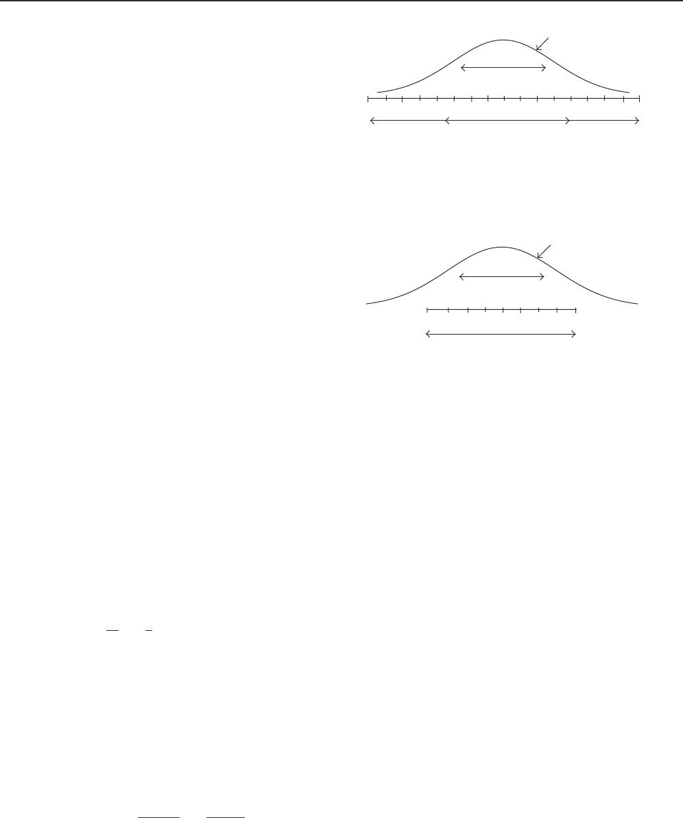
that maximizes capacity
Average power P
Quantized input le vels x
i
Square root of peak power E
c
Figure 1: Peak power of quantizer is larger than average power im-
posed.
Gaussian input distribution
that maximizes capacity
Average power P
Quantized input le vels x
i
Square root of peak power E
c
Figure 2: Peak power of quantizer is smaller than average power
imposed.
givenin(4), valid for an unquantized Gaussian channel with
average signal power constraint P? We also examine the in-
put distribution that achieves capacity in the quantized block
transmission channel.
We consider only the average power constraint P and as
a result we use two definitions for SNR in the presentation
of our simulation results in Section 3 . The first is the nomi-
nal SNR (P/σ
2
z
) already defined in (3), and the second is the
actual SNR (
x∈X
x
2
r(x)/σ
2
z
), where {X
⊆ X : r(x) =
0forallx ∈ X
}. From our simulation results in Section 3
we observe that the actual SNR is equal to the nominal SNR
if the peak power E
c
>P. Interestingly in [14], Var nica pro-
posed an approach that avoids the issue of nominal versus
actual SNR given that a subset X
of the inputs is already
chosen.
To examine the effect on capacity of the interaction be-
tween E
c
and P, we refer to Figures 1 and 2. Figure 1 shows a
regime where the peak power of the quantizer E
c
is much
larger than the average power imposed P. Because we are
interested in approaching the capacity of the unquantized
MIMO channel, which is achieved by a Gaussian distribu-
tion shown as the curve in the figure, to observe an approx-
imate Gaussian optimum input dist ribution in our quan-
tized system, we deliberately set E
c
>P. The so-called high-
resolution theory [16] covers the case where E
c
P and
there are fine quantization levels. However, it is unclear how
a coarse quantization affects further the performance. Our
results (see Section 3, Figure 6) show that whereas at high
SNR performance degrades more with precision loss than
with saturation loss, at low SNR and in the regime where
E
c
>P, we closely approach the Shannon bound inspite of
having a coarse quantization. In Figure 2 instead, E
c
<P.

4 EURASIP Journal on Advances in Signal Processing
Step (1) Compute p(y | x).
Initialize:
(1) Choose any r(x) such that 0 <r(x) < 1and
x
r(x) = 1.
(2) Initialize capacity C
0
, C
−1
.
Repeat until C
n
− C
n−1
≤ ε
,for some ε
≥ 0
Step (2) Compute:
(1) C
n−1
= C
n
.
(2) q
n
(x | y) = r
n−1
(x)p(y | x)/
x
r
n−1
(x)p(y | x).
(3) C
n
=
x
y
r
n−1
(x)p(y | x)logq
n
(x | y)/r
n−1
(x).
Step (3) Initialize the parameter β : β
0,n
, β
−1,n
.
Repeat until β
i,n
− β
i−1,n
≤ ε
,forsomeε
≥ 0
Step (4) Compute:
(1) β
i−1,n
= β
i,n
.
(2) β
i,n
= β
i−1,n
−
xe
β
i
−1,n
x
2
[1−x
2
/P]
y
q
n
(x|y)
p(y|x)
/
x
x
2
e
β
i−1,n
x
2
1 −x
2
/P
·
y
q
n
(x | y)
p(y|x)
end
Step (5) Compute:
r
n
(x) = e
β
n
x
2
y
q
n
(x | y)
p(y|x)
/
x
e
β
n
x
2
y
q
n
(x
| y)
p(y|x
)
.
end
Algorithm 1: The constrained Blahut-Arimoto algorithm.
In this regime the average power constraint is loose and the
modified Blahut-Arimoto algorithm utilizes all inputs and
assigns input probabilities as if the average power constraint
was not in place. This results in a maximizing input distri-
bution which departs from the Gaussian one. Simulation re-
sults in Sections 3 and 4 show as expected that the perfor-
mancedegradescomparedtotheanalogchannelaswemove
away from the Gaussian distribution case, because the ra-
tio of peak-to-average power reduces. Thus by increasing the
ratio of peak-to-average power, we are stil l within the con-
straints of (3), yet we come arbitrarily close to achieving the
Shannon capacity bound at low SNR.
2.1. Algorithm for computing the capacity of
a block transmission channel with
quantized inputs and outputs
Let r(x) denote the input distribution of the channel symbols
and let p(y
| x) denote the channel transition probability
which is a function of SNR, where SNR is defined as P/σ
2
z
.
1
q(x | y) denotes the conditional distribution of x given
y. The constrained Blahut-Arimoto algorithm we use for
computing the capacity of the quantized block transmission
channel is derived below and summarized in Algorithm 1.
1
Since we are given H and x, the channel transition probability is actually
p(y
| Hx). Given Hx, y ∼ N (Hx , σ
2
z
I), thus knowing the quantization
levels and appropriate decision regions, the complementary error func-
tion can be used to compute p(y
| Hx)[9].
Derivation of algorithm
Using the earlier defined quantities r(x), p(y
| x), and q(x |
y), we want to obtain the capacity C of the channel given by
C
= max
r(x)
I(X; Y)
= max
q(x |y)
max
r(x)
x
y
r(x)p(y | x)log
q(x
| y)
r(x)
(6)
subject to the constraints
x
r(x) = 1, (7)
x
x
2
r(x) ≤ P. (8)
Start with an initial guess for r(x). The maximizing condi-
tional distribution q(x
| y)isgivenby[5–8, 14, 17]
q(x
| y) =
r(x)p(y | x)
x
r(x)p(y | x )
. (9)
Given constraints (7)and(8), we obtain (6) using Lagrange
multipliers as a maximization of
I(X; Y)
=
x
y
r(x)p(y | x)log
q(x
| y)
r(x)
+ λ
x
r(x) − 1
+ β
x
x
2
r(x) − P
=
x
y
r(x)p(y | x)log
q(x
| y)
r(x)
+ λ
x
r(x) − λ + β
x
x
2
r(x) − βP.
(10)
Maximizing I(X; Y)withrespecttor(x), we obtain
∂I(X; Y)
∂r(x)
=
y
p(y | x)log
q(x
| y)
r(x)
−
y
r(x)p(y | x)
1
r(x)
+ λ + β
x
2
= 0
(11)
which implies that
y
p(y | x)log
q(x
| y)
r(x)
− 1+λ + βx
2
= 0. (12)
Thus
e
1−λ
e
−βx
2
= e
y
log [q(x|y)/r(x)]
p(y|x)
= r(x)
(−
y
p(y|x))
y
q(x | y)
p(y|x)
,
(13)
r(x)
=
y
q(x | y)
p(y|x)
e
1−λ
e
−βx
2
. (14)

O. Ndili and T. Ogunfunmi 5
If we substitute for r(x)in(7), we obtain
1
=
x
y
q(x | y)
p(y|x)
e
1−λ
e
−βx
2
=⇒ e
1−λ
=
x
y
q(x | y)
p(y|x)
e
−βx
2
.
(15)
If we substitute for r(x)in(8), we obtain
P
≥
x
x
2
y
q(x | y)
p(y|x)
e
1−λ
e
−βx
2
(16)
which implies that
1
≥
x
x
2
P
·
y
q(x | y)
p(y|x)
e
1−λ
e
−βx
2
. (17)
Combining (15)and(17)weobtain
x
e
βx
2
y
q(x | y)
p(y|x)
≥
x
x
2
P
e
βx
2
y
q(x | y)
p(y|x)
.
(18)
Thus
x
1 −
x
2
P
e
βx
2
y
q(x | y)
p(y|x)
≥ 0, (19)
where (19) is a nonlinear equation in β which we solve nu-
merically using the Newton-Raphson method. This yields an
iterative solution for β given by
β
n+1
= β
n
−
x
e
β
n
x
2
1 −x
2
/P
y
q(x | y)
p(y|x)
x
x
2
e
β
n
x
2
1 −x
2
/P
y
q(x | y)
p(y|x)
,
(20)
where n is the index of iteration. In Section 2.4 we will deter-
mine a reasonable initial guess for β.
2
With a solution for β,
the optimum input distribution is then given as
r(x)
=
e
βx
2
y
q(x | y)
p(y|x)
x
e
βx
2
y
q(x
| y)
p(y|x
)
(21)
by combining (14)and(15).
2.2. A specific case
When computing the capacity of a block transmission chan-
nel with quantized inputs and real outputs as in a downlink
dial-up channel, (9) remains unchanged while (14)becomes
r(x)
=
e
log q(x|y)
p(y|x)
dy
e
1−λ
e
−βx
2
. (22)
2
Note that because we use the Newton-Raphson method for the numerical
solution of β, the right initial guess of β is crucial to avoid the convergence
of β to some unreasonable value that would yield unreasonable results or
in some cases, infinite iterations of the algorithm.
This follows by rewriting the first line of (13)as
e
1−λ
e
−βx
2
= e
log [q(x|y)/r(x)]
p(y|x)
dy
= e
log q(x|y)
p(y|x)
dy−
log r(x)
p(y|x)
dy
=
e
log q(x|y)
p(y|x)
dy
r(x)
.
(23)
Simple manipulation of (23)yields(22).
Substituting this value for r(x)in(14) and using simi-
lar computations as was done from (15)to(21), we finally
obtain r(x)as
r(x)
=
e
βx
2
e
log q(x|y)
p(y|x)
dy
x
e
βx
2
e
log q(x|y)
p(y|x)
dy
. (24)
For the purposes of implementation, it is acceptable to
quantize the output Y into bins of length ΔY,whereΔY is
small compared to the variance of the noise σ
2
z
and ΔY ≤ ΔX.
Consider
ζ
=
log q(x | y)
p(y|x)
dy
=
p(y | x)log
p(y
| x)r(x)
x
p(y | x)r(x)
dy
=
p(y | x)log
p(y
| x)
x
p(y | x)r(x)
dy +logr(x).
(25)
Noting that
p(y
| x) =
1
2πσ
2
z
M
e
−y−Hx
2
/2σ
2
z
= ξe
−y−x
2
/2σ
2
z
,
(26)
we see that
ζ
= log ξ + ξ
e
−y−Hx
2
/2σ
2
z
·
−
y − Hx
2
2σ
2
z
dy
−
p(y | x)log
x
p(y | x)r(x)dy +logr(x)
= log ξ − σ
2
z
+logr(x) −
p(y | x)log
x
p(y | x)r(x)dy.
(27)
Finally we consider
p(y | x)log
x
p(y | x)r(x)dy.Wenote
that
x
p(y | x )r(x) is a weighted sum of exponentials that
are shifted in their mean. T his yields a function that is
Reimann integrable provided the variance Var(Y
| X ) = σ
2
z
is finite > 0. If the quantization of X is fine enoug h, the
smoothness of
x
p(y | x)r(x)dy increases especially at low
SNR. Therefore we can approximate the continuous output Y
by a quantized output as long as the number of quantization
levels is greater than or equal to the number of quantization
levels of the input.

6 EURASIP Journal on Advances in Signal Processing
2.3. Convergence
References [8, 18, 19 ] have shown that the Blahut-Arimoto
algorithm converges with a speed that is at least inversely
proportional to the approximation error (ε
). The Newton-
Raphson method used to obtain β in (20) has also been
shown to converge to a local root, given that the initial value
is sufficiently close to the desired root [20]. While we offer no
formal proof that our algorithm converges, empirical results
from our simulations show that it does. In the follow ing sub-
section, we define an appropriate initial guess for β.Thecon-
vergence speed of the Newton-Raphson method is quadratic
in ε
.
2.4. Analysis
In this section we determine a reasonable initial guess for β.
In our bid to design systems with information rates arbitrar-
ily close to the Shannon capacit y bound shown in (4), it is
useful for us to also examine how the capacity of the chan-
nel is affected by the average power constraint P and by the
number of levels of the quantizer.
Result
Given the par ameters λ and β from the constrained optimiza-
tion of I(X; Y), where λ and β are both functions of p(y
| x),
the following result holds:
1
− λ − βP = I(X ; Y). (28)
Proof. We start by rewriting (14)as
log r(x )
= log
y
q(x | y)
p(y|x)
− log e
1−λ−βx
2
= λ − 1+βx
2
+
y
p(y | x)log
p(y
| x)r(x)
p(y)
= λ − 1+βx
2
+
y
p(y | x)logp(y | x)
+logr(x)
y
p(y | x) −
y
p(y | x)logp(y)
(29)
which means that
1
− λ − βx
2
=
y
p(y | x)logp(y | x)
−
y
p(y | x)logp(y).
(30)
If we multiply both sides of (30)byr(x)andsumoverallx,
we obtain (28).
As P →∞, I(X; Y) tends to the capacity achieved by the
unconstrained Blahut-Arimoto algorithm which can be at
most log
2
|X| bits/use of the channel. Since β is introduced
in the maximization of (10) through the power constraint P,
0.12
0.1
0.08
0.06
0.04
0.02
0
β
2 4 6 8 10 12 14 16
Number of iterations for solving β
Figure 3: Typical convergence pattern of β.
this implies that as P increases, β decreases. In other words,
the effect of β is greater as the power constraint becomes
stricter. Because of this, a reasonable initial guess of β
0
for
(20)is0.Forβ
0
= 0, (20)becomes
β
1
= 0 −
x
1 −x
2
/P
y
q(x | y)
p(y|x)
x
x
2
1 −x
2
/P
y
q(x | y)
p(y|x)
. (31)
Note that we can conclude from (31) that β is negative as
P
→∞because at some stage, x
2
≤ P for all x ∈ X.
Indeed β is negative for all values of P because r(x)andβ
satisfy the first order Kuhn-Tucker conditions for obtaining
the unique, global optimum of a concave function subject to
concave constraints. These conditions are
∂I(X; Y)
∂r(x)
= 0; r(x) ≥ 0,
∂I(X; Y)
∂β
≤ 0; β ≤ 0,
(32)
fromwhichweseethatβ is negative. Figure 3 is a plot show-
ing the typical convergence pattern of β from our simulation
results. Values of β are seen to be negative. Figure 4 shows
that β decreases as SNR increases.
At the low SNR region, the maximizing input distribu-
tion tends towards a Gaussian distribution. We can see this
by utilizing high-resolution analysis [16]
I(X
Δ
; Y
Δ
) ≈ I(X; Y), as Δ −→ 0, (33)
where Δ is the quantization step, I(X
Δ
; Y
Δ
) is the mutual
information between the quantized versions of the random
variables X and Y,andI(X; Y) is the information rate of
the unquantized block transmission channel which is max-
imized by a Gaussian input distribution. It is p ermissible to
use high-resolution analysis for the low SNR reg ion because
in this region we are constrained from peaks that are so far
from the mean of the distribution that in essence E
c
→∞.
O. Ndili and T. Ogunfunmi 7
0.12
0.11
0.1
0.09
0.08
0.07
0.06
0.05
0.04
0.03
0.02
β
10 5 0 5 10152025
SNR (dB)
E
c
= 2P
E
c
= 3P
Figure 4: Variation of β with SNR.
Also Δ → 0 compared to the standard deviation of the noise
because at low SNR, the standard deviation of the noise is
large and the input is independent of the noise. The com-
bined conditions of Δ
→ 0andE
c
→∞yield the high-
resolution scenario.
Figures 7 and 10 are simulation results which show that
the maximizing input distribution at low SNR is concave like
the Gaussian distribution. We conclude that at low SNR, the
capacity of the quantized block transmission channel will be
closer to the Shannon bound.
As to the effect on information rate, of number of quan-
tization levels of the quantizer, high-resolution analysis [16,
21] implies that as Δ
→ 0 (i.e., as number of quantization
levels increases), approximately optimal per formance on a
Gaussian channel can be obtained.
In our case however, because SNR presents a constraint,
the high-resolution scenario cannot be realized. Another way
of looking at this is stating that we c annot arbitrarily increase
the number of quantization levels and still utilize all the avail-
able input signals because at some stage, satisfactory error
performance can no longer be achieved (by uncoded modu-
lation) [10]. Hence the goal of our analysis was to find a way
to approximate the high-resolution scenario given the dual
constraints of a per missible SNR and a specific channel al-
phabet.
From our analysis we propose that given average power P,
peak power E
c
, and the quantization levels, the performance
of the quantized block transmission channel a pproaches that
of the analog channel when we constrain the quantized block
transmission channel to approximate the analog channel, by
increasing peak-to-average power ratio.
In the next sections we present simulation results which
support our claims, and thereby present important underly-
ing principles behind designing a quantized block tr a nsmis-
sion system that achieves capacity close to that of an unquan-
tized block transmission system in the low SNR region.
0
0.5
1
1.5
2
2.5
3
3.5
4
4.5
Rates (bits/channel use)
10 50 510152025
SNR (dB)
Comparison of capacities of SISO channel
Unquantized channel
4-bit quantized channel, E
c
= 3P
3-bit quantized channel, E
c
= 3P
3-bit quantized channel, E
c
= 2P
3-bit quantized channel, E
c
= P
Figure 5: Comparison of capacity versus nominal SNR for different
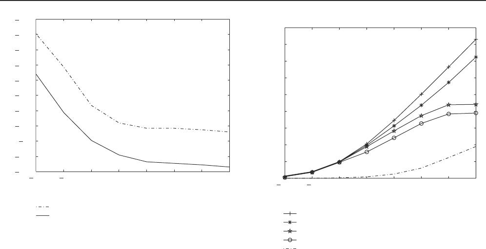
SISO channels.
3. RESULTS: CAPACITY OF SISO CHANNEL
We run simulations in which we arbitrarily generate the
channel impulse response h
l
in (1) and then run Algorithm 1.
Our simulations show the comparison of the capacities of the
following channels: 4 bit (16-level) quantized SISO channel
with E
c
= 3P, 3 bit quantized SISO channel with E
c
= 3P,
3 bit quantized SISO channel with E
c
= 2P,3bitquan-
tized SISO channel with E
c
= P, and the unquantized SISO
channel. Figure 5 shows the capacity curves for these chan-
nels plotted against nominal SNR (P/σ
2
z
). Figure 5 shows
the same curves plotted against actual average SNR achieved
(
x∈X
x
2
r(x)/σ
2
z
), from which we see that the actual SNR
achieved is affected by the value of E
c
used and the nominal
SNRismorelikelytobeachievedwhenE
c
>P.
From Figure 5 we see that as the ratio of peak-to-
average power increases, we approach more closely the ca-
pacity achieved by the unquantized channel. Also the per-
formance improves with increased number of input levels.
High-resolution analysis does not provide information on
how reduced peak-to-average ratio (saturation loss) and re-
duced number of quantization levels (precision loss) affect
the performance of the channel, relative to each other. From
Figure 6, we see that performance degrades more with preci-
sion loss than with saturation loss. This is expected because
for any given value of E
c
, you can do better by increasing the
number of quantization levels whereas if you fix the number
of quantization levels and increase E
c
, you cannot do b et-
ter beyond a certain value due to the fact that the number
of inputs are only so many. Note also that the precision gain
depends on the SNR and is much lower at low SNR. We can
see in addition that at low SNR the information rate is almost
8 EURASIP Journal on Advances in Signal Processing
0
0.5
1
1.5
2
2.5
3
3.5
4
4.5
Rates (bits/channel use)
25 20 15 10 5 0 5 10152025
Average SNR (dB)
Comparison of capacities of SISO channel
Unquantized channel
4-bit quantized channel, E
c
= 3P
3-bit quantized channel, E
c
= 3P
3-bit quantized channel, E
c
= 2P
3-bit quantized channel, E
c
= P
Figure 6: Comparison of capacity versus actual SNR for different
SISO channels.
0
0.02
0.04
0.06
0.08
0.1
0.12
0.14
0.16
Input probability
10 50 5101520
Inputs
Figure 7: Maximizing input distribution at low SNR for the SISO
channel.
insensitive to precision loss and is dominated instead by satu-
ration loss (the slope of the curve is higher for a higher peak-
to-average ratio). Note that the slope of the cur ves is a func-
tion of the number of quantization levels (it is the same for
equal number of quantization levels). The results obtained
from our simulations therefore support our earlier discus-
sions.
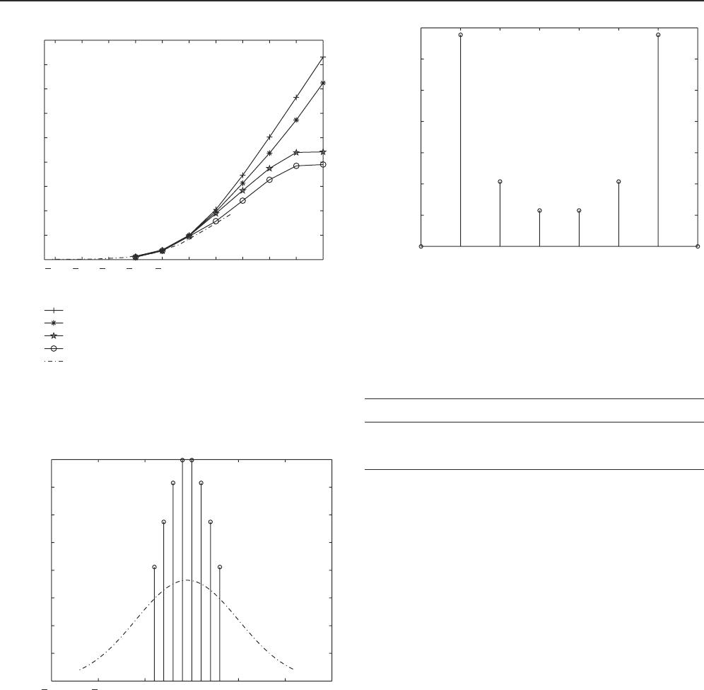
Figure 7 shows a typical maximizing input distribution
at low SNR and Figure 8 shows a maximizing input distr i-
bution at high SNR. These figures show that the maximizing
0
0.05
0.1
0.15
0.2
0.25
0.3
0.35
Input probability
12345678
Inputs
Figure 8: A maximizing input distribution at high SNR for the
SISO channel.
Table 1: Accuracy of predicted value of capacity as SNR increases.
SNR CC
−10 dB 0.0621 0.0410
−5dB 0.1838 −0.0827
input distribution tends further away from Gaussian as P in-
creases as was discussed in Section 2 . If we approximate the
maximizing distribution at low SNR by quantizing an appro-
priate Gaussian distribution (as shown in Figure 7), then we
can predict the capacity at this SNR and our predictions will
be fair.
This is shown by Table 1 where we see that the predicted
capacity C
is close to the actual capacity C at low SNR
but the prediction is poorer as SNR increases because the
maximizing input distribution is far from Gaussian. In the
next section, we present results of similar simulations for the
block transmission (MIMO) channel.
4. RESULTS: CAPACITY OF MIMO CHANNEL
Similar to our simulations for the SISO channel, we run sev-
eral simulations for the MIMO channel and for each simula-
tion, we randomly generate the circulant matrix H, then im-
plement Algorithm 1. Again we take the average capacity ob-
tained from our simulations. For reasons of computational
complexity we consider channel length L
= 2andsymbol
block length M
= 3. Channel memory order 1 is reasonable
for our example application, the dial-up channel, because the
frequency response of the analog twisted copper pair is al-
most flat over the 4 KHz bandwidth used for transmission.
We show the results of comparing the capacities of
the following channels: 4-level, 3-dimensional (M
= 3),
quantized MIMO channel with E
c
= 3P, 4-level, 3-
dimensional quantized MIMO channel with E
c
= 2P, 4-level,

O. Ndili and T. Ogunfunmi 9
0
0.5
1
1.5
2
2.5
3
3.5
4
4.5
5
Rates (bits/channel use)
10 50 510152025
SNR (dB)
Comparison of capacities of MIMO channel
Unquantized channel
5-level quantized channel, E
c
= 3P
4-level quantized channel, E
c
= 3P
4-level quantized channel, E
c
= 2P
4-level quantized channel, E
c
= P
Figure 9: Comparison of capacity versus nominal SNR for different
MIMO channels.
0
0.05
0.1
0.15
0.2
0.25
0.3
0.35
Input probability
11.522.53 3.54
Inputs
Figure 10: A maximizing input distribution at low SNR for the
MIMO channel.
3-dimensional quantized MIMO channel with E
c
= P,5-
level, 3-dimensional quantized MIMO channel with E
c
= 3P,
and the unquantized MIMO channel. Figure 9 shows the ca-
pacity curves for these channels plotted against nominal SNR
(P/σ
2
z
). We observe a gain that as with the SISO case, per-
formance improves with increased peak-to-average ratio and
increased number of quantization levels. The marginal dis-
tribution of a typical maximizing input distribution for the
quantized MIMO channel at low SNR is shown in Figure 10.
As we would expect, the marginal distribution is concave like
the Gaussian distribution.
xTU-C
(In-line sections)
9kftof
26 AWG
1.5kftof
24 AWG
50 ft of
drop wire
xTU-R
PSTN
0.5kftof
24 AWG
User
(Bridge tap section)
Figure 11: A typical end-to-end loop.
16
15.5
15
14.5
14
13.5
Loss in dB
00.511.522.533.54
10
3
MHz
Frequency response of typical loop
Figure 12: Frequency response of a typical end-to-end loop.
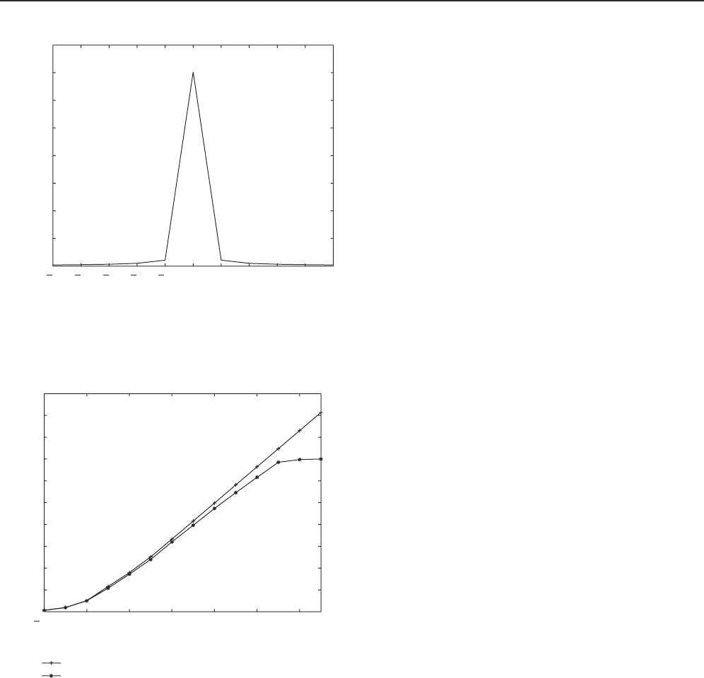
5. A PRACTICAL EXAMPLE
It is interesting to apply the capacity bounds developed in
this paper to a practical example which is the downlink chan-
nel of a dial-up connection, where the inputs are quantized
and the outputs are real. In this section we will simulate prac-
tical line conditions for a typical downlink dial-up channel
[22]. The end-to-end loop we analyze is shown in Figure 11.
The transfer function of the loop is given in [22]andcanbe
calculated using published tables which are also provided in
[22]. The bandwidth of interest is 3600 Hz between 150 Hz
and 3750 Hz. This is the bandwidth that allows optimum
performance. The frequency response obtained is shown in
Figure 12. Figure 13 is the impulse response of the end-to-
end loop. In our simulations, we assume the input X is uni-
formly quantized into 128 levels. In practice, the input con-
stellation is picked to approach a uniform quantization as
closely as possible [23]. The channel is sampled at a rate of
8000 Hz. We choose as average power P, the FCC-imposed
average transmit power P
=−12 dBm, we set E
c
= 3P and,
we vary the noise power σ
2
z
.AnSNRvalueofaround55dB
is expected under normal operating conditions [23]. We use
block length M
= 3 and the length of the channel impulse
response L = 2.TheresultweobtainisshowninFigure 14.
10 EURASIP Journal on Advances in Signal Processing
0
0.005
0.01
0.015
0.02
0.025
0.03
0.035
0.04
Impulse response
5 4 3 2 1012345
Taps
Impulse response of a typical loop
Figure 13: Impulse response of a typical end-to-end loop.
0
1
2
3
4
5
6
7
8
9
10
Rate (bits/dimension)
100 1020304050
SNR, P/σ
2
z
(dB)
Capacity of V.90 downstream
Unquantized channel
Quantized channel
Figure 14: Capacity of the downstream link.
From Figure 14 we can see that at low SNR, the capacity
of the quantized channel approaches the capacity of the un-
quantized channel very closely and at an SNR of about 45dB,
the Nyquist rate of the channel 56 kbps (
= 7 bits/dimension
× 8000 dimensions/s) is achieved under the prevailing line
conditions. This shows that the limit of 53.3kbpscanbeim-
proved upon.
6. CONCLUSION
In this paper we have in general, proposed useful guide-
lines for the design of block transmission systems whose
performance at low SNR is arbitrarily close to the Shannon
bound. Specifically, we have tested our proposals by apply ing
them to the downlink channel of a dial-up system and found
that we improved upon the limit of 53.3kpbs.
ACKNOWLEDGMENTS
The authors would like to thank Professor Anna Scaglione of
Cornell University, New York, for her valuable contributions
to this work and the Editor and Reviewers of this journal for
their useful comments.
REFERENCES
[1] E. Ayanoglu, N. R. Dagdeviren, G. D. Golden, and J. E. Mazo,
“An equalizer design technique for the PCM modem: a new
modem for the digital public switched network,” IEEE Trans-
actions on Communications, vol. 46, no. 6, pp. 763–774, 1998.
[2]D.J.Rauschmayer,ADSL/VDSL Principles : A Practical and
Precise Study of Asymmetric Digital Subscriber Lines and Ve ry
High Speed Digital Subscriber Lines,Macmillan,NewYork,NY,
USA, 1999.
[3] D. S. Lawyer, “Modem-HOWTO,” May 2003, http://www.tldp.
org/HOWTO/Modem-HOWTO-1.html.
[4] C. E. Shannon, “A mathematical theory of communications,”
Bell Systems Technical Journal, vol. 27, pp. 379–423 (pt I), 623–
656 (pt II), 1948.
[5] S. Arimoto, “An algorithm for computing the capacity of ar-
bitrary discrete memoryless channels,” IEEE Transactions on
Information Theory, vol. 18, no. 1, pp. 14–20, 1972.
[6] R. E. Blahut, “Computation of channel capacity and rate-
distortion functions,” IEEE Transactions on Information The-
ory, vol. 18, no. 4, pp. 460–473, 1972.
[7] A. Kavcic, “On the capacity of Markov sources over noisy
channels,” in Proceedings of the IEEE Global Telecommunica-
tions Conference (GLOBECOM ’01), vol. 5, pp. 2997–3001, San
Antonio, Tex, USA, November 2001.
[8] N. Varnica, X. Ma, and A. Kavcic, “Capacity of power con-
strained memoryless AWGN channels with fixed input con-
stellations,” in Proceedings of the IEEE Global Telecommuni-
cations Conference (GLOBECOM ’02), vol. 2, pp. 1339–1343,
Taip ei, Taiwan, November 2002.
[9] B. Honary, F. Ali, and M. Darnell, “Information capacity of
additive white Gaussian noise channel with practical con-
straints,” IEEProceedings,PartI:Communications,Speechand
Vision, vol. 137, no. 5, pp. 295–301, October 1990.
[10] G. Ungerboeck, “Channel coding with multilevel/phase sig-
nals,” IEEE Transactions on Information Theory, vol. 28, no. 1,
pp. 55–67, 1981.
[11] L. H. Ozarow and A. D. Wyner, “On the capacity of the Gaus-
sian channel with a finite number of input levels,” IEEE Trans-
actions on Information Theory, vol. 36, no. 6, pp. 1426–1428,
1990.
[12] S.Shamai(Shitz),L.H.Ozarow,andA.D.Wyner,“Informa-
tion rates for a discrete-time Gaussian channel w ith intersym-
bol interference and stationary inputs,” IEEE Transactions on
Information Theory, vol. 37, no. 6, pp. 1527–1539, 1991.
[13] N. Varnica, X. Ma, and A. Kavcic, “Power-constrained mem-
or yless and intersymbol interference channels with finite in-
put alphabets: capacities and concatenated code construc-
tions,” to appear in IEEE Transactions on Communications,
http://hrl.harvard.edu/
∼varnica/publications.htm.
